5. Geo Services Guide
This guide covers the details of geo data management and retrieval in rasdaman. The rasdaman Array DBMS is domain agnostic; the specific semantics of space and time is provided through a layer on top of rasdaman, historically known as petascope. It offers spatio-temporal access and analytics through APIs based on the OGC data standard Coverage Implementation Schema (CIS) and the OGC service standards Web Map Service (WMS), Web Coverage Service (WCS), and Web Coverage Processing Service (WCPS).
Note
While the name petascope addresses a specific component we frequently use the name rasdaman to refer to the complete system, including petascope.
5.1. OGC Coverage Standards Overview
For operating rasdaman geo services as well as for accessing such geo services through these APIs it is important to understand the mechanics of the relevant standards. In particular, the concept of OGC / ISO coverages is important.
In standardization, coverages are used to represent space/time varying phenomena, concretely: regular and irregular grids, point clouds, and general meshes. The coverage standards offer data and service models for dealing with those. In rasdaman, focus is on multi-dimensional gridded (“raster”) coverages.
In rasdaman, the OGC standards WMS, WCS, and WCPS are supported, being reference implementation for WCS. These APIs serve different purposes:
WMS delivers a 2D map as a visual image, suitable for consunmption by humans
WCS delivers n-D data, suitable for further processing and analysis
WCPS performs flexible server-side processing, filtering, analytics, and fusion on coverages.
These coverage data and service concepts are summarized briefly below. Ample material is also available on the Web for familiarization with coverages (best consult in this sequence):
hands-on demos for multi-dimensional coverage services provided by Constructor University;
a series of webinars and tutorial slides provided by EarthServer;
a range of background information on these standards provided by OGC;
the official standards documents maintained by OGC:
5.1.1. Coverage Data
OGC CIS specifies an interoperable, conformance-testable coverage structure independent from any particular format encoding. Encodings are defined in OGC in GML, JSON, RDF, as well as a series of binary formats including GeoTIFF, netCDF, JPEG2000, and GRIB2).
By separating the data definition (CIS) from the service definition (WCS) it is possible for coverages to be served throuigh a variety of APIs, such as WMS, WPS, and SOS. However, WCS and WCPS have coverage-specific functionality making them particularly suitable for flexible coverage acess, analytics, and fusion.
5.1.2. Coverage Services
OGC WMS delivers 2D maps generated from styled layers stacked up. As such, WMS is a visualization service sitting at the end of processing pipelines, geared towards human consumption.
OGC WCS, on the other hand, provides data suitable for further processing (including visualization); as such, it is suitable also for machine-to-machine communication as it appears in the middle of longer processing pipelines. WCS is a modular suite of service functionality on coverages. WCS Core defines download of coverages and parts thereof, through subsetting directives, as well as delivery in some output format requested by the client. A set of WCS Extensions adds further functionality facets.
One of those is WCS Processing; it defines the ProcessCoverages request
which allows sending a coverage analytics request through the WCPS
spatio-temporal analytics language. WCPS supports extraction, analytics, and
fusion of multi-dimensional coverage expressed in a high-level, declarative, and
safe language.
5.2. OGC Web Services Endpoint
Once the petascope geo service is deployed (see rasdaman installation
guide) coverages can be accessed through the HTTP
service endpoint /rasdaman/ows.
For example, assuming that the service IP address is 123.456.789.1 and the
service port is 8080, the following request URLs would deliver the
Capabilities documents for OGC WMS and WCS, respectively:
http://123.456.789.1:8080/rasdaman/ows?SERVICE=WMS&REQUEST=GetCapabilities&VERSION=1.3.0
http://123.456.789.1:8080/rasdaman/ows?SERVICE=WCS&REQUEST=GetCapabilities&VERSION=2.0.1
Text responses, e.g. for GetCapabilities request, will be compressed for faster download
if the client sends the request with HTTP header Accept-Encoding: gzip.
This is normally automatically done by the browser, but may need to be
explicitly handled when developing clients or from using command-line tools.
5.3. OGC Coverage Implementation Schema (CIS)
A coverage consists mainly of:
domain set: provides information about where data sit in space and time. All coordinates expressed there are relative to the coverage’s Coordinate Reference System or Native CRS. Both CRS and its axes, units of measure, etc. are indiciated in the domain set. Petascope currently supports grid topologies whose axes are aligned with the axes of the CRS. Along these axes, grid lines can be spaced regularly or irregularly.
range set: the “pixel payload”, ie: the values (which can be atomic, like in a DEM, or records of values, like in hyperspectral imagery).
range type: the semantics of the range values, given by type information, null values, accuracy, etc.
metadata: a black bag which can contain any data: the coverage will not understand these, but duly transport them along so that the connection between data and metadata is not lost.
Further components include Envelope which gives a rough, simplified overview
on the coverage’s location in space and time and CoverageFunction which is
unused by any implementation known to us.
5.3.1. Coverage CRS
Every coverage, as per OGC CIS, must have exactly one native Coordinate Reference System (CRS), which is given by a URL. Resolving this URL should deliver the CRS definition. The OGC CRS resolver is an example of a public service for resolving CRS URLs; the same service is also bundled in every rasdaman installation, so that it is avialable locally. More details on this topic can be found in the CRS Management chapter.
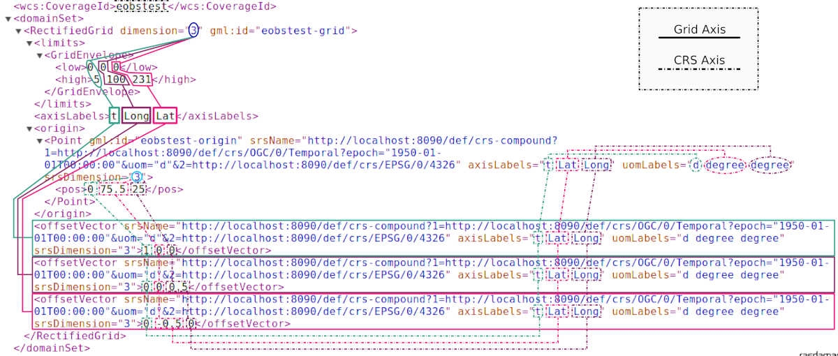
Sometimes definitions for CRSs are readily available, such as the 2-D WGS84 with code EPSG:4326 in the EPSG registry. In particular spatio-temporal CRSs, however, are not always readily available, at least not in all combinations of spatial and temporal axes. To this end, composition of CRS is supported so that the single Native CRS can be built from “ingredient” CRSs by concatenating them into a composite one. For instance, a time-series of WGS84 images would have the following Native CRS:
http://localhost:8080/def/crs-compound?
      1=http://localhost:8080/def/crs/OGC/0/AnsiDate
     &2=http://localhost:8080/def/crs/EPSG/0/4326
Coordinate tuples in this CRS represent an ordered composition of a temporal
coordinate expressed in ISO 8601 syntax, such as 2012-01-01T00:01:20Z,
followed by latitude and longitude coordinates, as per EPSG:4326.
The native CRS of a coverage domain set can be determined in severay ways:
in a WCS
GetCapabilitiesresponse, thewcs:CoverageSummary/ows:BoundingBox@crsattribute;in a WCS
DescribeCoverageresponse, thesrsNameattribute in thegml:domainSetelement; Furthermore, theaxisLabelsattribute contains the CRS axis names according to the CRS sequency, and theuomLabelsattribute contains the units of measure for each corresponding axis.in WCPS, the function
crsSet(e)returns the CRS of a coverage expression e;
The following graphics illustrates, on the example of an image timeseries,
how dimension, CRS, and axis labels affect the domain set in
a CIS 1.0 RectifiedGridCoverage.
Note
This handling of coordinates in CIS 1.0 bears some legacy burden from GML;
in the GeneralGridCoverage introduced with CIS 1.1 coordinate handling is
much simplified.
5.3.2. Range Type
Range values can be atomic or (possibly nested) records over atomic values, described by the range type. In rasdaman the following atomic data types are supported; all of these can be combined freely in records of values, such as in hyperspectral images or climate variables.
rasdaman type |
size |
Quantity types |
|---|---|---|
|
8 bit |
unsignedByte |
|
8 bit |
signedByte |
|
8 bit |
unsignedByte |
|
16 bit |
signedShort |
|
16 bit |
unsignedShort |
|
32 bit |
signedInt |
|
32 bit |
unsignedInt |
|
32 bit |
float32 |
|
64 bit |
float64 |
|
64 bit |
cfloat32 |
|
128 bit |
cfloat64 |
5.3.3. Nil Values
Nil (null) values, as per SWE, are supported by rasdaman in an extended way:
null values can be defined over any data type
nulls can be single values
nulls can be intervals
a null definnition in a coverage can be a list of all of the above alternatives.
Full details can be found in the null values section.
Note
It is highly recommended to NOT define single null values over floating-point data as this causes numerical problems well known in mathematics. This is not related to rasdaman, but intrinsic to the nature and handling of floating-point numbers in computers. A floating-point interval around the desired float null value should be preferred (this corresponds to interval arithmetics in numerical mathematics).
5.3.4. Errors
Errors from OGC requests to rasdaman are returned to the client formatted as
ows:ExceptionReport (OGC Common Specification).
An ExceptionReport can contain multiple Exception elements.
For example, when running a WCS GetCoverage or a WCPS query which execute
rasql queries in rasdaman, in case of an error the ExceptionReport will contain
two Exception elements:
One with the error message returned from rasdaman.
Another with the rasql query that failed.
For example:
<ows:ExceptionReport>
    <ows:Exception exceptionCode="RasdamanRequestFailed">
        <ows:ExceptionText>The Encode function is applicable to array arguments only.</ows:ExceptionText>
    </ows:Exception>
    <ows:Exception exceptionCode="RasdamanRequestFailed">
        <ows:ExceptionText>Failed internal rasql query: SELECT encode(1, "png" ) FROM mean_summer_airtemp AS c</ows:ExceptionText>
    </ows:Exception>
</ows:ExceptionReport>
5.4. OGC Web Coverage Service
WCS Core offers the following request types:
GetCapabilitiesfor obtaining a list of coverages offered together with an overall service description;DescribeCoveragefor obtaining information about a coverage without downloading it;GetCoveragefor downloading, extracting, and reformatting of coverages; this is the central workhorse of WCS.
WCS Extensions in part enhance GetCoverage with additional functionality
controlled by further parameters, and in part establish new request types,
such as:
WCS-T defining
InsertCoverage,DeleteCoverage, andUpdateCoveragerequests;WCS Processing defining
ProcessCoveragesfor submitting WCPS analytics code.
You can use http://localhost:8080/rasdaman/ows as service endpoints to which to
send WCS requests, for example:
http://localhost:8080/rasdaman/ows?service=WCS&version=2.0.1&request=GetCapabilities
Examples to send GetCoverage requests with curl client as
HTTP GET and POST to petascope:
5.4.1. Subsetting behavior
This section describes how rasdaman translates geo-referenced coordinates (e.g. in spatio-temporal subsets) to internal grid coordinates, which are required in the internal rasql queries generated for each geo request.
This is particular to regular geo axes of a coverage. The behavior for irregular axes is explained here.
5.4.1.1. Terminology
General
geo axis - a geo-referenceable axis of a coverage, e.g. Lat, Lon, time, etc.
grid axis - an axis referenceable with grid (integer) coordinates; internally geo axis coordinates have to be translated to grid integer coordinates
subset - a list of trims and/or slices
trim - a pair of lower and upper bounds indicating a range on a geo axis
slice - a single coordinate on a geo axis
Rasdaman-provided information
axis_res- geo resolution (positive or negative) on a regular axisaxis_min- minimum geo axis boundaxis_max- maximum geo axis boundaxis_grid_min- minimum grid axis bound
User-provided information
subset_min- minimum trim geo bound, or a slice coordinatesubset_max- maximum trim geo bound (none if it is a slicing operation)
5.4.1.2. Preconditions
Valid trims on a geo axis must fulfill the following precondition:
axis_min <= subset_min <= subset_max <= axis_max
Valid slices on a geo axis must fulfill the following preconditions:
if
axis_res > 0thenaxis_min <= subset_min < axis_maxif
axis_res < 0thenaxis_min < subset_min <= axis_max
Furthermore, for irregular axes:
Slicing: exactly one of the axis coefficients must be equal to the slice coordinate
subset_min, or a coefficient’s area of validity (if defined) must intersect it.Trimming: at least one of the axis coefficients must be within the
[subset_min, subset_max]interval, or at least one coefficient’s area of validity (if defined) must intersect it.
5.4.1.3. Geo-to-grid coordinate translation
Translating geo coordinates to grid coordinates on a regular axis is done with the formula below. It is assumed that the preconditions in the previous section are already satisfied.
# 1. A small value is extracted from subset_max to emulate right-open interval.
#    It cannot be fixed as it eventually becomes ineffective at certain magnitudes;
#    for that reason it is scaled to the resolution.
epsilon = abs(axis_res) * 1e-11

# 2. Handle Axis Y (e.g. Lat) with negative axis_res = opposite behavior:
#    swap coordinates and limits; this allows to use the same formula in 3a/b
#    below for both positive and negative resolution.
if axis_res < 0:
    epsilon *= -1
    # the origin for negative resolution is the upper subset/axis bound
    swap subset_min and subset_max
    swap axis_min and axis_max

# 3a. Calculate grid low bound
grid_min_tmp = (subset_min - axis_min) / axis_res
if grid_min_tmp != floor(grid_min_tmp) and grid_min_tmp < 0:
   # for axis with negative resolution and grid min is a float number, it needs to be adjusted
   # e.g. -5.00000000000001 should be shifted to -5 instead of -6
   grid_min_tmp = grid_min_tmp + abs(epsilon)

# *floor* is used to make sure that the result is an integer grid coordinate;
# some rounding method must be used, and floor works well with left-closed interval.
# NOTE: axis_grid_min is used because the axis grid lower bound is not always 0.
grid_min =  axis_grid_min + floor( grid_min_tmp )

# 3b. Calculate grid high bound
if subset_min != subset_max:
    # The formula is analogous to the one above for grid_min, but
    # we extract a small epsilon from subset_max to emulate right-open interval.
    grid_max = axis_grid_min + floor( ((subset_max - epsilon) - axis_min) / axis_res )

# 4. Output of the formula
if subset_min != subset_max:
  return (grid_min, grid_max) # trim
else:
  return grid_min             # slice
Example. The following subset performs slicing on the Lat and trimming
on the Lon axis of coverage $c in WCPS: $c[Lat(-89.0), Lon(0.0, 180.0)].
The formula values provided by rasdaman are as follows:
Axis
Lon:axis_res=1, axis_min=-180, axis_max=180, axis_grid_min=0Axis
Lat:axis_res=-1, axis_min=-90, axis_max=90, axis_grid_min=0
The formula would return the following grid indices:
Lat(-89.0) -> 179Lon(0.0, 180.0) -> (170, 359)
5.4.2. CIS 1.0 to 1.1 Transformation
Under WCS 2.1 - ie: with SERVICE=2.1.0 - both DescribeCoverage and
GetCoverage requests understand the proprietary parameter
OUTPUTTYPE=GeneralGridCoverage which formats the result as CIS 1.1
GeneralGridCoverage even if it has been imported into the server as a CIS
1.0 coverage, for example:
http://localhost:8080/rasdaman/ows?SERVICE=WCS&VERSION=2.1.0
    &REQUEST=DescribeCoverage
    &COVERAGEID=test_mean_summer_airtemp
    &OUTPUTTYPE=GeneralGridCoverage

http://localhost:8080/rasdaman/ows?SERVICE=WCS&VERSION=2.1.0
    &REQUEST=GetCoverage
    &COVERAGEID=test_mean_summer_airtemp
    &FORMAT=application/gml+xml
    &OUTPUTTYPE=GeneralGridCoverage
5.4.3. Polygon/Raster Clipping
WCS and WCPS support clipping of polygons expressed in the
WKT format format.
Polygons can be MultiPolygon (2D), Polygon (2D) and LineString (1D+).
The result is always a 2D coverage in case of MultiPolygon and Polygon, and
is a 1D coverage in case of LineString.
Further clipping patterns include curtain and corridor on 3D+ coverages
from Polygon (2D) and Linestring (1D). The result of curtain
clipping has the same dimensionality as the input coverage whereas the result of
corridor clipping is always a 3D coverage, with the first axis being the
trackline of the corridor by convention.
In WCS, clipping is expressed by adding a &CLIP= parameter to the
request. If the SUBSETTINGCRS parameter is specified then this CRS also
applies to the clipping WKT, otherwise it is assumed that the WKT is in the
Native coverage CRS. In WCPS, clipping is done with a clip function, much
like in rasql.
Further information can be found in the rasql clipping section. Below we list examples illustrating the functionality in WCS and WCPS.
5.4.3.1. Clipping Examples
Polygon clipping on coverage with Native CRS
EPSG:4326, for example:WCS:
WCPS:
Polygon clipping with coordinates in
EPSG:3857(fromsubsettingCRSparameter) on coverage with Native CRSEPSG:4326, for example:WCS:
WCPS:
Linestring clipping on a 3D coverage with axes
X,Y,ansidate, for example:WCS:
WCPS:
Multipolygon clipping on 2D coverage, for example:
WCS:
WCPS:
Curtain clipping by a Linestring on 3D coverage, for example:
Curtain clipping by a Polygon on 3D coverage, for example:
Corridor clipping by a Linestring on 3D coverage, for example:
Corridor clipping by a Polygon on 3D coverage, for example:
Note
Subspace clipping is not supported in WCS or WCPS.
5.4.4. Areas of validity on irregular axes
By default, coefficients on an irregular axes act as single points: subsetting on such an axis must specify exactly the coefficient (slice), or contain the coefficient itself in the lower/upper bounds (trim).
It is possible to customize this behavior when importing data by specifying areas of validity which extend the coefficients from single points into intervals with a start and an end; this concept is also known as footprints or sample space. Refer to the corresponding import documentation on how to specify the areas of validity.
The areas of validity specify a closed interval [start, end] around each
coefficient on an irregular axis, such that start <= coefficient <= end.
Areas of validity may not overlap.
The start and end may be specified with less than millisecond precision, e.g.
"2010" and "2012-05". In this case they are expanded to millisecond
precision internally such that start is the earliest possible datetime
starting with "2010" (i.e. "2010-01-01T00:00:00.000Z") and end is the
latest possible datetime starting with "2012-05"
(i.e. "2012-05-31T23:59:59.999Z"). The same semantics applies in
subsetting in queries, see Temporal subsets.
The effect on subsetting is as follows:
slicing: a coordinate
Cwill select the coefficient with area of validity that intersectsC. For example if the coefficient is"2010"(resolved when importing in petascope as"2010-01-01T00:00:00.000Z") and its area of validity has start"2009-01-01"and end"2011-12-31", then slicing at coordinate"2009-05-01"will return the coefficient, as will at"2010-12-31", and anything else between the start and (not including) the end.trimming: an interval
lo:hiwill select all coefficients with areas of validity that intersect or are contained in the[lo,hi]interval.
If a coverage was imported with custom areas of validity, they will be listed in
the WCS DescribeCoverage response under XML element
<ras:covMetadata>. A <ras:axes> element contains <ras:axis> child
element for each coverage axis wth areas of validity which are then listed
as <ras:areasOfValidity> children with start and end attributes, e.g:
5.4.5. WCS-T
Currently, WCS-T supports importing coverages in GML format. The metadata of the coverage is thus explicitly specified, while the raw cell values can be stored either explicitly in the GML body, or in an external file linked in the GML body, as shown in the examples below. The format of the file storing the cell values must be
2-D data supported by the GDAL library, such as TIFF / GeoTIFF, JPEG / JPEG2000, PNG, etc;
n-D data in NetCDF or GRIB format
In addition to the WCS-T standard parameters petascope supports additional proprietary parameters, covered in the following sections.
Note
For coverage management normally WCS-T is not used directly. Rather, the more
convenient wcst_import Python tool is recommended for Data Import.
5.4.5.1. Inserting coverages
Inserting a new coverage into the server’s WCS offerings is done using the
InsertCoverage request.
Request Parameter |
Value |
Description |
Required |
|---|---|---|---|
SERVICE |
WCS |
service standard |
Yes |
VERSION |
2.0.1 or later |
WCS version used |
Yes |
REQUEST |
InsertCoverage |
Request type to be performed |
Yes |
INPUTCOVERAGEREF |
{url} |
URl pointing to the coverage to be inserted |
One of inputCoverageRef or inputCoverage is required |
INPUTCOVERAGE |
{coverage} |
A coverage to be inserted |
One of inputCoverageRef or inputCoverage is required |
USEID |
new | existing |
Indicates wheter to use the coverage’s id (“existing”) or to generate a new unique one (“new”) |
No (default: existing) |
Request Parameter |
Value |
Description |
Required |
|---|---|---|---|
PIXELDATATYPE |
GDAL supported base data type (eg: “Float32”) or comma-separated concatenated data types, (eg: “Float32,Int32,Float32”) |
In cases where range values are given in the GML body the datatype can be indicated through this parameter. Default: Byte. |
No |
TILING |
rasdaman tiling clause, see Storage Layout Language |
Indicates the array tiling to be applied during insertion |
No |
The response of a successful coverage request is the coverage id of the newly inserted coverage. For example: The coverage available at http://schemas.opengis.net/gmlcov/1.0/examples/exampleRectifiedGridCoverage-1.xml can be imported with the following request:
http://localhost:8080/rasdaman/ows?SERVICE=WCS&VERSION=2.0.1
    &REQUEST=InsertCoverage
    &COVERAGEREF=http://schemas.opengis.net/gmlcov/1.0/examples/exampleRectifiedGridCoverage-1.xml
The following example shows how to insert a coverage stored on the server on which rasdaman runs. The cell values are stored in a TIFF file (attachment:myCov.gml), the coverage id is generated by the server and aligned tiling is used for the array storing the cell values:
http://localhost:8080/rasdaman/ows?SERVICE=WCS&VERSION=2.0.1
    &REQUEST=InsertCoverage
    &COVERAGEREF=file:///etc/data/myCov.gml
    &USEID=new
    &TILING=aligned[0:500,0:500]
5.4.5.2. Updating Coverages
Updating an existing coverage into the server’s WCS offerings is done using the UpdateCoverage request.
Request Parameter |
Value |
Description |
Required |
|---|---|---|---|
SERVICE |
WCS |
service standard |
Yes |
VERSION |
2.0.1 or later |
WCS version used |
Yes |
REQUEST |
UpdateCoverage |
Request type to be performed |
Yes |
COVERAGEID |
{string} |
Identifier of the coverage to be updated |
Yes |
INPUTCOVERAGEREF |
{url} |
URl pointing to the coverage to be inserted |
One of inputCoverageRef or inputCoverage is required |
INPUTCOVERAGE |
{coverage} |
A coverage to be updated |
One of inputCoverageRef or inputCoverage is required |
SUBSET |
AxisLabel(geoLowerBound, geoUpperBound) |
Trim or slice expression, one per updated coverage dimension |
No |
The following example shows how to update an existing coverage test_mr_metadata
from a generated GML file by wcst_import tool:
http://localhost:8080/rasdaman/ows?SERVICE=WCS&version=2.0.1
    &REQUEST=UpdateCoverage
    &COVRAGEID=test_mr_metadata
    &SUBSET=i(0,60)
    &subset=j(0,40)
    &INPUTCOVERAGEREF=file:///tmp/4514863c_55bb_462f_a4d9_5a3143c0e467.gml
5.4.5.3. Deleting Coverages
The DeleteCoverage request type serves to delete a coverage (consisting of
the underlying rasdaman collection, the associated WMS layer (if exists)
and the petascope metadata).
For example: The coverage test_mr can be deleted as follows:
http://localhost:8080/rasdaman/ows?SERVICE=WCS&VERSION=2.0.1
    &REQUEST=DeleteCoverage
    &COVERAGEID=test_mr
5.4.6. Renaming a coverage
The /rasdaman/admin/coverage/update non-standard API allows to update a
coverage id and the associated WMS layer if one exists (v10.0+). For example,
the coverage test_mr can be renamed to test_mr_new as follows:
http://localhost:8080/rasdaman/admin/coverage/update
    ?COVERAGEID=test_mr
    &NEWCOVERAGEID=test_mr_new
5.4.7. Update coverage metadata
Coverage metadata can be updated through the interactive rasdaman WSClient on
the OGC WCS > Describe Coverage tab, by selecting a text file (MIME type must
be one of text/xml or text/plain) containing the
new metadata; Note that to be able to do this it is necessary to login first in
the Admin tab.
The non-standard API for this feature is at /rasdaman/admin/coverage/update
which operates through multipart/form-data POST requests. The request should
contain 2 parts:
the
coverageIdto update, andthe path to a local text file to be uploaded to the server.
For example, the below request will update the metadata of coverage
test_mr_metadata with the one in a local XML file at
/home/rasdaman/Downloads/test_metadata.xml by using the curl tool:
curl --form-string "COVERAGEID=test_mr_metadata"
     -F "file=@/home/rasdaman/Downloads/test_metadata.xml"
     "http://localhost:8080/rasdaman/admin/coverage/update"
5.4.8. Update coverage’s null values
Coverage’s null values can be updated via the non-standard API at
/rasdaman/admin/coverage/nullvalues/update endpoint
with two mandatory parameters:
coverageId: the name of the coverage to be updatednullvalues: null values of coverage’s band(s) with the format corresponding to rasql, see syntax doc.
Note
Value of nullvalues must be encoded in clients properly
for special characters such as: [, ], {, }.
Example of using curl tool to update null values
of a 3-bands coverage:
curl 'http://localhost:8080/rasdaman/admin/coverage/nullvalues/update'
    -d 'COVERAGEID=test_rgb&NULLVALUES=[35, 25:35, 35:35]'
    -u rasadmin:rasadmin
5.4.9. Update coverage range type
The rangeType of a coverage can be updated via the
/rasdaman/admin/coverage/rangetype/update endpoint API
with two mandatory parameters:
coverageId: the name of the coverage to be updatedrangeType: XML string describes coverage’s bands in (Sensor Web Enablement) SWE standards, with root element is<swe:dataRecord>>.
Example of using curl tool to update coverage’s range type
of a 2-bands coverage to one band as swe:Quantity and one band as swe:Category:
updated_range.xml file contains these content:

<swe:DataRecord>
        <swe:field name="Band1">
            <swe:Quantity definition="http://www.opengis.net/def/dataType/OGC/0/UnsignedInt">
                <swe:label>Band 1 label</swe:label>
                <swe:description>Band 1 description</swe:description>
                <swe:nilValues>
                    <swe:NilValues>
                        <swe:nilValue reason="Null by no data">25</swe:nilValue>
                    </swe:NilValues>
                </swe:nilValues>
                <swe:uom code="10^0"/>
            </swe:Quantity>
        </swe:field>
        <swe:field name="Band2">
            <swe:Category definition="Band 2 definition which is an attribute">
                <swe:description/>
                <swe:nilValues>
                    <swe:NilValues>
                        <swe:nilValue reason="Null value from interval">25:35</swe:nilValue>
                        <swe:nilValue reason="Null value from a single value">57</swe:nilValue>
                    </swe:NilValues>
                </swe:nilValues>
                <swe:codeSpace xlink:href="http://code.list.org/"/>
            </swe:Category>
        </swe:field>
    </swe:DataRecord>


curl -u rasadmin:rasadmin \
  'http://localhost:8080/rasdaman/admin/coverage/rangetype/update' \
  --data-urlencode COVERAGEID=test_cov \
  --data-urlencode RANGETYPE@updated_range.xml
5.4.10. Convert irregular axis to regular axis
This feature allows to convert a suitable irregular axis to a regular axis, when the irregular axis has equal distances between its coefficients. Typical use case is to convert an irregular time axis with daily / hourly coefficients to regular time axis with time step (time resolution) = day / hour.
The endpoint API is /rasdaman/admin/coverage/update
with three mandatory parameters:
coverageId: name of the coverage to be updatedaxis: name of the irregular axis to be convertednewtype: only possible value isRegularAxis
Example of using the curl command-line tool to convert the axis
ansi in a coverage test_cov to a regular axis:
curl -u rasadmin:rasadmin 'http://localhost:8080/rasdaman/admin/coverage/update' \
     -d "COVERAGEID=test_cov&axis=ansi&newtype=RegularAxis"
5.4.11. Update regular axis’ origin
This feature allows to update an existing regular axis’ origin in a coverage, which effective changes the geo lower and upper bounds of this axis. It is used in the case when the geo bounds of an regular axis are shifted to some unwanted values after coverage imported, and the admin wants to update them to proper values.
The endpoint API is /rasdaman/admin/coverage/update
with three mandatory parameters:
coverageId: name of the coverage to be updatedaxis: name of the regular axis to be updatedorigin: the new origin of the axis. It can be in ISO Datetime format (e.g."1960-12-31T12:00:00.000Z") if axis is temporal or number (e.g.23.5) in other cases.Note
New geo bounds are calculated in petascope based on the origin like below.
If axis’ resolution is positive (e.g. lon, E, X, AnsiDate,…) then:
newGeoLowerBound = origin - 0.5 * resolution
newGeoUpperBound = newGeoLowerBound + total_grid_pixels * resolution
If axis’ resolution is negative (e.g. lat, N, Y,…) then:
newGeoUpperBound = origin + 0.5 * abs(resolution)
newGeoLowerBound = newGeoUpperBound + total_grid_pixels * resolution
Example of using the curl command-line tool to update origin of axis
ansi with resolution=1 day in a coverage test_cov.
Before updating, extent of axis is: ["1960-12-31T12:00:00.000Z":"2024-06-24T12:00:00.000Z"].
After udpating, extent of axis is: ["1960-01-01T00:00:00.000Z":"2024-06-25T00:00:00.000Z"].
curl -u rasadmin:rasadmin 'http://localhost:8080/rasdaman/admin/coverage/update' \
     -d 'COVERAGEID=test_cov&axis=ansi&origin="1961-01-01T12:00:00.000Z"'
5.4.12. INSPIRE Coverages
The INSPIRE Download Service is an implementation of the Technical Guidance for the implementation of INSPIRE Download Services using Web Coverage Services (WCS) version 2.0+.
In order to achieve INSPIRE Download Service compliance, the following enhancements
have been implemented in rasdaman for WCS GetCapabilities response.
Under
<ows:OperationsMetadata>there is a new section for INSPIRE metadata for the service. For example, the result below contains two INSPIRE coveragescov_1andcov_2.Service Metadata URL field (
<inspire_common:URL>), a URL containing the location of the metadata associated with the WCS service which is configured by settinginspire_common_urlinpetascope.properties.Under
<inspire_common:SupportedLanguages>section, the supported language is fixed toeng(English) only.A coverage is considered INSPIRE coverage, if it has a specific URL set by
metadataURL attribute. All INSPIRE coverages is listed in the list of XML elements<inspire_dls:SpatialDataSetIdentifier>. The example above contains two INSPIRE coverages, each<inspire_dls:SpatialDataSetIdentifier>element containing an attribute metadataURL to provide more information about the coverages. The value for<inspire_common:Namespace>elements of each INSPIRE coverage is derived from the service endpoint.
5.4.12.1. Create an INSPIRE coverage
Controlling whether a local coverage is treated as an INSPIRE coverage can be done by:
Manually sending a request to
/rasdaman/admin/inspire/metadata/updatewith two mandatory parameters:COVERAGEID- the coverage to be converted to an INSPIRE coverageMETADATAURL- a URL to an INSPIRE-compliant catalog entry for this coverage; if set to empty, i.e.METADATAURL=then the coverage is marked as non-INSPIRE coverage.
For example, the coverage
test_inspire_metadatacan be marked as INSPIRE coverage as follows:curl --user rasadmin:rasadmin -X POST \ --form-string 'COVERAGEID=test_inspire_metadata' \ -F 'METADATAURL=https://inspire-geoportal.ec.europa.eu/16.iso19139.xml' \ 'http://localhost:8080//rasdaman/admin/inspire/metadata/update'Via
wcst_import.sh, in an ingredients files with inspire section contains the settings for importing INSPIRE coverage:metadata_url- If set to non-empty string, then the importing coverage will be marked as INSPIRE coverage. If set to empty string or omitted, then the coverage will be updated as non-INSPIRE coverage.
For example, the coverage
cov_3will be imported as INSPIRE coverage with this configuration in the ingredients file:
5.4.13. Coverage thumbnail
Each coverage can have a thumbnail, a small PNG or JPEG image that provides a
quick visual overview of the coverage. To get the thumbnail of a coverage
<coverageId> (no credentials required):
http://localhost:8080/rasdaman/ows/coverage/thumbnail?COVERAGEID=<coverageId>
If the coverage has a thumbnail, then the image will be returned.
If the coverage has no thumbnail but has an associated WMS layer, then rasdaman will use a WMS
GetMaprequest to render the most recent temporal slice as an image of size 250 x 250. If the request has no credentials and server requires authentication, then petascope throws HTTP 404 error.Otherwise, an exception is thrown.
A thumbnail can be set by:
Add
thumbnail_pathsetting in the wcst_import ingredients file when importing a new coverage (docs)A request to the
/rasdaman/admin/coverage/thumbnail/updateAPI withCOVERAGEIDparameter for the coverage ID, and the thumbnail image for parameterTHUMBNAILGRAPHIC:# NOTE: An @ character preceding the image file path is required in order to upload its contents curl -u rasadmin:rasadmin 'http://localhost:8080/rasdaman/admin/coverage/thumbnail/update' -F 'COVERAGEID=test_wms_4326' -F 'THUMBNAILGRAPHIC=@/tmp/thumbnail.jpg'
Alternatively, the image file could be converted to a
base64text string and uploaded as follows:# NOTE: the file size that can generally be uploaded in this way # is limited to about 100 kB, depending on OS limits for command-line # argument sizes. coverage_id="test_coverage" thumbnail="/tmp/thumnail_image.png" format=$(file "$thumbnail" | grep -iEo 'jpeg|png' | head -n1 | tr '[:upper:]' '[:lower:]') base64_str=$(base64 -w 0 "$thumbnail") base64_final="data:image/$format;base64,$base64_str" api_url="http://localhost:8080/rasdaman/admin/coverage/thumbnail/update" curl -u 'rasadmin:rasadmin' "$api_url?COVERAGEID=$coverage_id" \ -d "THUMBNAILGRAPHIC=$base64_final"
In either case, it is recommended for the thumbnail to be an image of size 250x250 pixels.
5.4.14. Check if a coverage exists
Rasdaman offers non-standard API to check if a coverage exists in a
simpler and faster way than doing a GetCapabilities or a DescribeCoverage
request. The result is a true/false string literal.
Example:
http://localhost:8080/rasdaman/admin/coverage/exist?coverageId=cov1
5.4.15. GetCapabilities response extensions
The WCS GetCapabilities response contains some rasdaman-specific extensions,
as documented below.
The
<ows:AdditionalParameters>element of each coverage contains some information which can be useful to clients:sizeInBytes- an estimated size (in bytes) of the coveragesizeInBytesWithPyramidLevels- an estimated size (in bytes) of the base coverage plus sizes of its pyramid coverages; only available if this coverage has pyramidaxisList- the coverage axis labels in geo CRS order
Example:
5.4.16. DescribeCoverage rasdaman metadata
Rasdaman may generate specific metadata in the DescribeCoverage response for a particular coverage; this section documents the structure of this metadata.
If areas of validity were defined during the import of a coverage, then they will be listed under an
<axes>element for each affected axis. More details on the metadata structur can be found here.If global metadata was specified explicitly or harvested automatically from input files during data import (docs), it will be listed in this section with multiple elements per metadata key/value pair. Each element has a name under the ras: namespace set to the key, and text content set to the value. For example, explicit metadata in the ingredients file specified like this:
"metadata": {
  "global": {
    "title": "ERA5-Land monthly averaged data from 1950 to present",
    "data_type": "Gridded"
  }
}
will appear as follows in the DescribeCoverage:
<ras:covMetadata>
  <ras:title>ERA5-Land monthly averaged data from 1950 to present</ras:title>
  <ras:data_type>Gridded</ras:data_type>
</ras:covMetadata>
If a color palette table was specified explicitly or harvested automatically from input files during data import (docs), it will be listed under a
<ras:colorPaletteTable>element. An example of color palette table and metadata (see previous point) collected from the input file:Listed with
gdalinfo, the file has the following metadata:If band and axis metadata has been specified explicitly or harvested automatically from input files during data import (docs), they will be listed under
<ras:bands>and<ras:axes>elements respectively. An axisAwill be a separate element<ras:A>, containing the axis metadata elements; it works the same for the coverage bands. For example, the import ingredients configuration listed in the example here will result in the following DescribeCoverage structure:
5.4.17. GetCoverage request
5.4.17.1. Interpolation
There are two supported formats for interpolation parameter in WCS GetCoverage requests:
Full URI, e.g.
http://www.opengis.net/def/interpolation/OGC/1.0/bilinearShort hand format, e.g.
bilinear
5.4.18. CRS notation
When a CRS is used in WCS / WCPS request for doing subsetting or projecting to an output CRS, these notations below are supported:
Full CRS URL, e.g.
http://localhost:8080/rasdaman/def/crs/EPSG/0/4326(standardized format)Shorthand CRS with authority, version and code, e.g.
EPSG/0/4326Shorthand CRS with authority and code, e.g.
EPSG:4326
5.5. OGC Web Coverage Processing Service (WCPS)
The OGC Web Coverage Processing Service (WCPS) standard defines a protocol-independent language for the extraction, processing, analysis, and fusion of multi-dimensional gridded coverages, often called datacubes.
5.5.1. General
WCPS requests can be submitted in both abstract syntax:
for c in (test_mean_summer_airtemp)
return
encode(c[Lat(-40:-35), Long(120:121)],
        "netcdf",
        "{ \"nodata\": [0], \"metadata\": { \"new_metadata\": \"This is a new added metadata\" }, \"formatParameters\": {\"INTERLEAVE\": \"BAND\"} }"
      )
and query embedded in XML wrapper elements:
<?xml version="1.0" encoding="UTF-8" ?>
    <ProcessCoveragesRequest xmlns="http://www.opengis.net/wcps/1.0" service="WCPS" version="1.0.0">
        <query>
            <abstractSyntax>
                for c in (test_mean_summer_airtemp)
                return
                    count(c[Lat(-43.525:-40), Long(125:130)] > 15) +
                    count(c[Lat(-43.525:-20), Long(125:150)] < 25)
            </abstractSyntax>
        </query>
    </ProcessCoveragesRequest>
For example, using the WCS GET/KVP protocol binding, a WCPS request can be sent
through the following ProcessCoverages request:
http://localhost:8080/rasdaman/ows?service=WCS&version=2.0.1
    &request=ProcessCoverage&query=<wcps-query>
The following subsections list enhancements rasdaman offers over the OGC WCPS standard. A brief introduction to the WCPS language is given in the WCPS cheatsheet; further educational material is available on EarthServer.
5.5.2. Polygon/Raster Clipping
The non-standard clip() function enables clipping in WCPS. The signature is
as follows:
clip( coverageExpression, wkt [, subsettingCrs ] )
where
coverageExpressionis an expression of result type coverage, e.g.dem + 10;wktis a valid WKT (Well-Known Text) expression, e.g.POLYGON((...)),LineString(...);subsettingCrsis an optional CRS URL in which thewktcoordinates are expressed, e.g."http://localhost:8080/rasdaman/def/crs/EPSG/0/4326".
5.5.2.1. Clipping Examples
Polygon clipping with coordinates in
EPSG:4326on coverage with native CRSEPSG:3857:Linestring clipping on 3D coverage with axes
X,Y,datetime.Linestring clipping on 2D coverage with axes
X,Y.In this case with
WITH COORDINATESextra parameter, the geo coordinates of the values on the linestring will be included as well in the result. The first two bands of the result holds the coordinates (by geo CRS order), and the remaining bands the original cell values. Example output for the above query:"-28.975 119.975 90","-28.975 120.475 84","-28.475 120.975 80", ...
Multipolygon clipping on 2D coverage.
Curtain clipping by a Linestring on 3D coverage
Curtain clipping by a Polygon on 3D coverage
Corridor clipping by a Linestring on 3D coverage
Corridor clipping by a Polygon on 3D coverage (geo CRS:
EPSG:4326) with input geo coordinates inEPSG:3857.
5.5.3. Auto-ratio for spatial scaling
The scale() function allows to specify the target extent of only one of the
spatial horizontal axes, instead of requiring both. In such a case, the extent
of the unspecified axis will be determined automatically while preserving the
original ratio between the two spatial axes.
For example in the request below, the extent of Lat will be automatically
set to a value that preserves the ratio in the output result:
5.5.4. Non-scaled axes are optional
The scale() function will implicitly add the full domains of unspecified
non-spatial axes of a given coverage, with the effect that they will not be
scaled in the result. This deviates from the OGC WCPS standard, which requires
all axes to be specified with target domains, even if the resolution of an axis
should not be changed in the result.
In the example query below, a 3D coverage is scaled only spatially because only
the spatial axes E and N are specified in the target scale intervals, while the
ansi non-spatial axis is omitted.
5.5.5. Extensions on domain functions
The domain interval can be extracted from a domain and imageCrsDomain.
Both the interval - ie: [lowerBound:upperBound] - and lower as well
as upper bound can be retrieved for each axis.
Syntax:
operator(.lo|.hi)?
with .lo or .hi returning the lower bound or upper bound of this interval.
Further, the third argument of the domain() operator, the CRS URL, is
optional. If not specified, domain() will use the CRS of the selected axis
(ie, the second argument) instead.
For example, the coverage AvgLandTemp has 3 dimensions with grid bounding
box of (0:184, 0:1799, 0:3599), and a geo bounding box of
("2000-02-01:2015-06-01", -90:90, -180:180). The table below lists various
expressions and their results:
Expression |
Result |
|---|---|
|
|
|
|
|
|
|
|
|
|
|
|
5.5.6. LET clause
An optional LET clause allows binding alias variables to valid WCPS query
sub-expressions; subsequently the alias variables can be used in the return
clause instead of repeating the aliased sub-expressions.
The syntax in context of a full query is as follows:
FOR-CLAUSE
LET $variable := assignment [ , $variable := assignment ]
   ...
[ WHERE-CLAUSE ]
RETURN-CLAUSE
where
assignment ::= coverageExpression | [ dimensionalIntervalList ]
An example with the first case:
for $c in (test_mr)
let $a := $c[i(0:50), j(0:40)],
    $b := avg($c) * 2
return
  encode( scale( $c, { imageCrsDomain( $c ) } ) + $b, "image/png" )
The second case allows to conveniently specify domains which can then be readily used in subset expression, e.g:
for $c in (test_mr)
let $dom := [i(20), j(40)]
return
  encode( $c[ $dom ] + 10, "itext/json" )
5.5.7. min and max functions
Given two coverage expressions A and B (resulting in compatible
coverages, i.e. same domains and types), min(A, B) and max(A, B)
calculate a result coverage with the minimum / maximum for each pair of
corresponding cell values of A and B.
For multiband coverages, bands in the operands must be pairwise compatible; comparison is done in lexicographic order with the first band being most significant and the last being least significant.
The result coverage value has the same domain and type as the input operands.
5.5.8. Positional parameters
Positional parameters allow to reference binary or string values in a WCPS
query, which are specified in a POST request in addition to the WCPS query.
Each positional parameter must be a positive integer prefixed by a $, e.g.
$1, $2, etc.
The endpoint to send WCPS query by POST with extra values is:
/rasdaman/ows?SERVICE=WCS&VERSION=2.0.1&REQUEST=ProcessCoverages
with the mandatory parameter query and optional positional parameters 1,
2, etc. The value of a positional parameter can be either a
binary file data or a string value.
5.5.8.1. Example
One can use the curl tool to send a WCPS request with
positional parameters from the command line; it will read the contents
of specified files automatically if they are prefixed with a @.
For example, to combine an existing coverage $c with two temporary coverages
$d and $e provided by positional parameters $1 and $2 into a
result encoded in png format (specified by positional parameter $3):
curl -s "http://localhost:8080/rasdaman/ows?SERVICE=WCS&VERSION=2.0.1&REQUEST=ProcessCoverages" \
     --form-string 'query=for $c in (existing_coverage), $d in (decode($1)), $e in (decode($2))
         return encode(($c + $d + $e)[Lat(0:90), Long(-180:180)], "$3"))' \
     -F "1=@/home/rasdaman/file1.tiff" \
     -F "2=@/home/rasdaman/file2.tiff" \
     -F "3=png" > test.png
Note
It is also possible to submit positional pararameters prefixed with $ character
when it is escaped as \$ in the bash command. For example:
curl ...
    -F "\$1=@/home/rasdaman/inputFile1.tiff" \
    -F "\$2=25.5"
5.5.9. Decode Operator in WCPS
The non-standard decode() operator allows to combine existing coverages with
temporary coverages created in memory from input files attached in the request
body via POST.
Only 2D geo-referenced files readable by GDAL are supported. One way to check if
a file $f is readable by GDAL is with gdalinfo $f. netCDF/GRIB
files are not supported.
5.5.9.1. Syntax
The syntax is
decode(${positional_parameter})
where ${positional_parameter) refers to files in the POST request.
See the previous section for more details
on positional parameters.
5.5.9.2. Example
5.5.10. Case Distinction
Conditional evaluation based on the cell values of a coverage is possible with
the switch expression. Although the syntax is a little different, the
semantics is very much compatible to the rasql case statement, so it is
recommended to additionally have a look at its corresponding
documentation.
5.5.10.1. Syntax
SWITCH
  CASE condExp RETURN resultExp
  [ CASE condExp RETURN resultExp ]*
  DEFAULT RETURN resultExpDefault
where condExp and resultExp are either scalar-valued or coverage-valued
expressions.
5.5.10.2. Constraints
All
condExpmust return either boolean values or boolean coveragesAll
resultExpmust return either scalar values, or coveragesThe domain of all condition expressions must be the same
The domain of all result expressions must be the same (that means same extent, resolution/direct positions, crs)
5.5.10.3. Evaluation Rules
If the result expressions return scalar values, the returned scalar value on a
branch is used in places where the condition expression on that branch evaluates
to True. If the result expressions return coverages, the values of the returned
coverage on a branch are copied in the result coverage in all places where the
condition coverage on that branch contains pixels with value True.
The conditions of the statement are evaluated in a manner similar to the IF-THEN-ELSE statement in programming languages such as Java or C++. This implies that the conditions must be specified by order of generality, starting with the least general and ending with the default result, which is the most general one. A less general condition specified after a more general condition will be ignored, as the expression meeting the less general expression will have had already met the more general condition.
Furthermore, the following hold:
domainSet(result)=domainSet(condExp1)metadata(result)=metadata(condExp1)rangeType(result)=rangeType(resultExp1). In case resultExp1 is a scalar, the result range type is the range type describing the coverage containing the single pixel resultExp1.
5.5.10.4. Examples
switch
  case $c < 10 return {red: 0;   green: 0;   blue: 255}
  case $c < 20 return {red: 0;   green: 255; blue:   0}
  case $c < 30 return {red: 255; green: 0;   blue:   0}
  default      return {red: 0;   green: 0;   blue:   0}
The above example assigns blue to all pixels in the $c coverage having a value less than 10, green to the ones having values at least equal to 10, but less than 20, red to the ones having values at least equal to 20 but less than 30 and black to all other pixels.
switch
  case $c > 0 return log($c)
  default     return 0
The above example computes log of all positive values in $c, and assigns 0 to the remaining ones.
switch
  case $c < 10 return $c * {red: 0;   green: 0;   blue: 255}
  case $c < 20 return $c * {red: 0;   green: 255; blue: 0}
  case $c < 30 return $c * {red: 255; green: 0;   blue: 0}
  default      return      {red: 0;   green: 0;   blue: 0}
The above example assigns blue: 255 multiplied by the original pixel value to all pixels in the $c coverage having a value less than 10, green: 255 multiplied by the original pixel value to the ones having values at least equal to 10, but less than 20, red: 255 multiplied by the original pixel value to the ones having values at least equal to 20 but less than 30 and black to all other pixels.
5.5.11. CIS 1.0 to CIS 1.1 encoding
For output format application/gml+xml WCPS supports delivery as CIS 1.1
GeneralGridCoverage by specifying an additional proprietary parameter
outputType in the encode() function, e.g:
for c in (test_irr_cube_2)
return encode( c, "application/gml+xml",
                  "{\"outputType\":\"GeneralGridCoverage\"}" )
5.5.12. Query Parameter
For specifying the WCPS query in a request, in addition to the query
parameter the non-standard q parameter is also supported. A request must
contain only one q or query parameter.
http://localhost:8080/rasdaman/ows?service=WCS&version=2.0.1
  &REQUEST=ProcessCoverage&q=<wcps-query>
5.5.13. Describe Operator in WCPS
The non-standard describe() function delivers a “coverage description” of a
given coverage without the range set, in either GML or JSON.
5.5.13.1. Syntax
describe( coverageExpression, outputFormat [ , extraParameters ] )
where
outputFormatis a string specifying the format encoding in which the result will be formatted. Formats are indicated through their MIME type identifier, just as inencode(). Formats supported:application/gml+xmlorgmlfor GMLapplication/jsonorjsonfor JSON
extraParametersis an optional string containing parameters for fine-tuning the output, just as inencode(). Options supported:"outputType=GeneralGridCoverage"to return a CIS 1.1 General Grid Coverage structure
5.5.13.2. Semantics
A describe() operation returns a description of the coverage resulting from
the coverage expression passed, consisting of domain set, range type, and
metadata, but not the range set. As such, this operator is the WCPS equivalent
to a WCS DescribeCoverage request, and the output adheres to the same WCS
schema.
The coverage description generated will follow the coverage’s type, so one of Rectified Grid Coverage (CIS 1.0), ReferenceableGridCoverage (CIS 1.0), or General Grid Coverage (CIS 1.0).
By default, the coverage will be provided as Rectified or Referenceable Grid
Coverage (in accordance with its type); optionally, a General Grid Coverage can
be generated instead through "outputType=GeneralGridCoverage". As JSON is
supported only from OGC CIS 1.1 onwards this format is only available (i) if the
coverage is stored as a CIS 1.1 General Grid Coverage (currently not supported)
or (ii) this output type is selected explicitly through an extraParameter.
Efficiency: The describe() operator normally does not materialize
the complete coverage, but determines only the coverage description making
this function very efficient. A full evaluation is only required
if coverageExpression contains a clip() performing a curtain, corridor,
or linestring operation.
5.5.13.3. Examples
Determine coverage description as a CIS 1.0 Rectified Grid Coverage in GML, without evaluating the range set:
for $c in (Cov)
return describe( $c.red[Lat(10:20), Long(30:40), "application/gml+xml" )
Deliver coverage description as a CIS 1.1 General Grid Coverage in GML, where range type changes in the query:
for $c in (Cov)
return describe( { $c.red; $c.green; $c.blue }, "application/gml+xml",
                                    "outputType=GeneralGridCoverage" )
Deliver coverage description as a CIS 1.1 General Grid Coverage, in JSON:
for $c in (Cov)
return describe( $c, "application/json", "outputType=GeneralGridCoverage" )
5.5.13.4. Specific Exceptions
Unsupported output format
This format is only supported for General Grid Coverage
Illegal extra parameter
5.5.14. Flip Operator in WCPS
The non-standard FLIP function enables reversing values from an axis
belonging to a coverage expression. The output coverage expression
has no changes in the grid domains, base type and dimensionality.
If encoded in gml format, then in gml:sequenceRule element,
the flipped axis shows its value with minus sign
(e.g. -1 instead of +1).
See more details in rasql.
Syntax
flipExp: FLIP coverageExpression ALONG axisLabel

axisLabel: identifier
A FLIP expression consists of coverageExpression which denotes the input coverage,
and one axisLabel of the coverage to flip values.
Examples
The following examples illustrate the syntax of the FLIP operator.
Flipping the 2D coverage expression on its
Longaxis, by using:for $c in (test_mean_summer_airtemp) return encode( FLIP $c[Lat(-30:-15), Long(125:145)] ALONG Long , "image/png")Flipping the 3D coverage expression on its
unixtime axis, by using:for $c in (test_wms_3d_time_series_irregular) return encode( FLIP $c[Lat(40:90), Long(80:140)] + 20 ALONG unix , "json")
5.5.15. Sort Operator in WCPS
The SORT operator enables the user to sort a coverage expression along an axis.
The sorting is done by slicing the array of the coverage along that axis, calculating a slice rank
for each of the slices, and then rearranging the slices according to their ranks,
in an ascending or descending order.
The sorting causes no change in the spatial domain, base type, or dimensionality. This means that the resulting array is the original array but with its values sorted at the sorting axis. See more details in rasql.
Note
After sorting, the geo domains (and coefficients for irregular axis) of the sorted axis are not changed, even though the grid values associated with geo coordinates are changed.
Syntax
sortExp: SORT coverageExp ALONG sortAxis [listingOrder] BY cellExp

coverageExp: a general coverage expression
sortAxis: identifier.
listingOrder: ASC (default if omitted) | DESC
cellExp: an expression that produces scalar ranks for each slice
along the sortAxis.
Note
One should not do subset (slice/trim) on the sortAxis in the cellExp
Examples
The following examples illustrate the syntax of the SORT operator.
Sort the 2D coverage expression on its
Lonaxis according to the coverage values at each longitude index and -40 latitude in ascending order:for $c in (test_mean_summer_airtemp) return encode( SORT $c ALONG Lon BY $c[Lat(-40)] , "image/png")Sort the 3D coverage expression on its
unixtime axis in descending order by the sum of each time slice along it:for $c in (test_wms_3d_time_series_irregular) return encode( SORT $c.Red + 30 ALONG unix DESC BY add($c) , "json")
5.5.16. Calendar capabilities
Since v10.3, rasdaman supports quite flexible and powerful methods for addressing temporal coordinates in WCS / WCPS subsetting and other operations. A common use case is aggregating data over a time series per temporal unit, e.g. per day, month, year, etc.
5.5.16.1. Temporal coordinates
Temporal coordinates must be specified in ISO datetime format; the full format
including all components is YYYY-MM-DDTHH:MM:SS.SSSZ, explained as follows:
YYYY: yearMM: monthDD: dayT: separator between date and time componentsHH: hourSS: secondSSS: milisecondZ: UTC timezone (GMT +0); imported coverages has a fixed timezone UTC currently, there is no support to change to different timezone when importing data
Not all components must be specified: at minimum YYYY is required.
The last component in the datetime value determines its granularity; for
example, the granularity of "2015-01-02" is day, while "2015-02" has
granularity month. The granularity modifies the range of a datetime string in
a subset. For example, the datetime value "2015-01" with
granularity month has a time range from lower bound
"2015-01-01T00:00:00:000Z" (first moment of January, 2015) to upper bound
"2015-01-31T23:59:59:999Z" (last moment of January, 2015).
5.5.16.2. Shifting temporal coordinates
It is possible to add or subtract a time period from a datetime value, thereby shifting the granularity as well. The shift period is specified separated by a whitespace after the datetime string. It is composed of several parts in sequence:
Initial designator
P(for Period): requiredNumber of years followed by
YNumber of months followed by
MNumber of days followed by
DTime designator (separator)
Trequired only if any time components are specifiedNumber of hours followed by
HNumber of minutes followed by
MNumber of seconds followed by
S
If any number is negative then the preceding datetime is shifted backward instead of forward as usual; non-required parts can be omitted.
For example, time("2015-01-01 P2Y") shifts the input datetime forward by 2
years to time("2017-01-01").
5.5.16.3. Concatenating time components
Individual time components can be concatenated into a full datetime string with
the . operator. Each component is either a string or a temporal function
which returns a string. For example time("2015" . "01" . "01") is a
slice which will be resolved as time("2015-01-01").
5.5.16.4. Temporal subsets
The semantics of slices and trims in temporal subsets is clarified subsequently.
Slicing generally selects a single index on a coverage axis. In temporal slices, however, we have to keep in mind the granularity of the datetime value.
If the time range defined by the granularity of the slice coordinate encompases exactly one grid index, then this index is returned.
Otherwise an error is returned, if it does not contain any grid index or contains more than one index. In this case it may be necessary to adjust the slicing to one with larger or smaller granularity, e.g. from
"2015-01"with month granularity to"2015-01-01"with day granularity.
Trimming corresponds to selecting all the indices between a lower and upper
bounds. On a temporal axis, the lower bound is converted to the full ISO
datetime format as before, while the upper bound is converted up to the last
moment of the granularity of the datetime value. For example, a trim
time("2015-01-01":"2015-01-03") is first expanded internally to
time("2015-01-01T00:00:00.000Z":"2015-01-03T23:59:59.999Z")
before it is used to subset the time axis.
For example, selecting only data in January 2023 could be done with
time("2023-01":"2023-01"); note that it is not necessary to specify any
further time components, e.g. day.
5.5.16.5. Time axis iterator
Coverage constructors and condensers have an OVER clause where iterator
variables over the coordinates of a coverage axis (potentially a subset) can be
specified. In case of a temporal axis, lists of temporal coordinates are built
from coverage domain information or time string literals. Afterwards, when the
constructor or condenser are evaluated, the iterator variable goes over the
list in sequence.
There are two ways to specify the temporal coordinates for iteration:
iterVar axis( "lowerBound" : "upperBound" [ : "step" ] )Here
lowerBoundandupperBoundare datetime values. Thestepis an optional parameter with same format as specified earlier in Shifting temporal coordinates, which indicates that theiterVarsteps from the lower to the upper bound instepincrements. Ifstepis omitted, then it is derived from the granularity of thelowerBound. For example,over $pt date("2014" : "2023" : "P1Y" )is identical toover $pt date("2014" : "2023"), as the granularity of the lower bound isP1Y; the iterated time coordinates will be"2014","2015", …,"2023".iterVar axis( "dateTime1", "dateTime2", ... )Here
iterVargoes through a list of explicitly specified datetime values. For example, this query will build a coverage of maximum values of the data slices at days explicitly listed in theoverclause:for c in (testCov) return encode( coverage result over $pt t("2023-01-01", "2023-01-02", "2023-01-03") values max ( c[t($pt : $pt)] ) , "csv")iterVar axis( timeTruncator(...) )The set of coordinates to iterate through is in this case generated by a time truncator function.
5.5.16.6. Time truncator functions
Time truncators allow to extract the actually present time coordinates, at a particular granularity, from a particular coverage under inspection. They are used typically in axis iterators of coverage constructor / general condenser.
They are a family of functions tr: list<datetime> -> list<datetime> which
reduce accuracy beyond the chosen granularity from all time stamps passed and
returns a set without duplicated values of matched datetimes; tr is one of
allyears, allmonths, alldays, allhours, allminutes, allseconds.
If $c is a coverage alias in a for clause, and its axis time extends
from 2022-11-01 to 2023-03-31, then:
allyears($c.domain.date)="2022","2023"allmonths($c.domain.date)="2022-11", …,"2023-03"alldays($c.domain.date)="2022-11-01", …,"2023-03-31"allhours($c.domain.date)="2022-11-01T00", …,"2023-03-30T23","2023-03-31T00"allminutes($c.domain.date)="2022-11-01T00:00", …,"2023-03-30T23:59","2023-03-31T00:00"allseconds($c.domain.date)="2022-11-01T00:00:00.000", ..,"2023-03-30T23:59.999","2023-03-31T00:00.000"
To iterate through all Januars in possible years on the time axis of a
coverage, we can write a query as follows:
for $c in (test_365_days_irregular)
return encode(

    coverage result
    over $pt date( allmonths( domain($c, time) ) )
    values $c[date($pt . "-01" : $pt . "-01")],

"json")
Here, allyears( domain($c, time) ) may return a list of "2022" and
"2023"; then for each $pt, date($pt . "-01" : $pt . "-01") will be
resolved as:
First iteration:
date("2022-01" : "2022-01")Second iteration:
date("2023-01" : "2023-01")
5.5.16.7. Time extractor functions
Time extractors allow to extract time components by a specified granularity in the used function name. They are used typically in axis iterators of coverage constructor / general condenser.
They are a family of functions s: list<datetime> -> list<numbers> which
return a set without duplicated values of time components contained in the
input list; s is one of years, months, days, hours, minutes, seconds.
If $c is a coverage alias in a for clause, and its axis time extends
from 2022-11-01 to 2023-03-31, then:
years(domain($c, time))="2022","2023"months(domain($c, time))="01","02","03","11","12"days(domain($c, time))="01", …,"31"hours(domain($c, time))="00", …,"23"minutes(domain($c, time))="00", …,"59"second(domain($c, time))="00.000", ..,"59.999"
For example, if the time axis is irregular with two indexes at
"2023-01-01" and "2023-08-01", then months( domain($c, time) ) in
the query below returns "01" and "08", and the iterated subsets in
date("2023-" . $m) will be "2023-01" and "2023-08":
for $c in (test_cov)
return encode(
       coverage temp_cov
       OVER $m date( months( domain($c, time) ) )
       VALUES $c[date("2023-" .  $m)],
"csv")
Another example: the time axis has daily coefficients over years 2020, 2021,
2022, 2023; this query will return all coefficients in February 2020:
for $c in (test_cov)
return encode(
       coverage temp_cov
       OVER $d date( days( domain($c[time("2020-02":"2020-02")], time) ) )
       VALUES $c[date("2020-02-" . $d)],
"csv")
Here, days( domain($c[time("2020-02":"2020-02")], time) returns
a set of 01","02",...,"29", and for each $d in the set
date("2020-02-" . $d) will be resolved as:
First iteration:
date("2020-02-01")Second iteration:
date("2020-02-02)…
Last iteration:
date("2020-02-29)
5.5.16.8. Incompatibilites
Prior to this calendar feature, subsets on a temporal axis is done like below:
Slice: e.g.
time("2015-01-01"), then this value is converted to ISO datetime format"2015-01-01T00:00:00.000Z"and the slice is applied on thetimeaxis. If this axis is irregular and it does not contain the coefficient at the above exact datetime, then petascope throws an exception because the coefficient is not found.Trim: e.g.
time("2015-01":"2015-12"), then the subset is converted to ISO datetime format as"2015-01-01T00:00:00:000Z":"2015-12-01T00:00:00:000Z"and iftimeaxis is irregular, then petascope will find any coefficients between these subsets and return them.
5.5.17. Polygonize function
This operation is useful in geographical context, providing ability to layer additional information on existing maps, for example. For more details, see also rasql polygonize.
When the result includes multiple files, as is the case with ESRI Shapefile,
the files will be compressed into a single zip archive.
Syntax
polygonize(covExp, targetFormat)
polygonize(covExp, targetFormat, connectedness)
Where
covExp: coverage expression
targetFormat: StringLit
connectedness: integerLit
Examples
The following WCPS query vectorizes a 2D geo-referenced coverage into shape file format:
for $c in (test_mean_summer_airtemp)
return
    polygonize($c, "ESRI Shapefile")
5.5.18. Concat operator in WCPS
The non-standard concat operator allows to glue coverage expressions
together along an axis to a coverage expression with a larger grid domain.
It is equivalent to concat in rasql with the same requirements
for grid domains of the contributing coverage expressions.
The result is a grid coverage without any geo-referencing metadata. The
concatenation axis in the along clause must exist in all concatenated
operand coverages.
Example
The following WCPS query concatenates two 1-D coverages
along axis j, creating a larger 1-D coverage:
for $c in (test_mr) return
encode(
        concat $c[i(0)] with $c[i(1)] along j
, "json")
5.6. OGC Web Map Service (WMS)
The OGC Web Map Service (WMS) standard provides a simple HTTP interface for requesting overlays of geo-registered map images, ready for display.
With petascope, geo data can be served simultaneously via WMS, WMTS, WCS, and WCPS. Further information:
This section mainly covers rasdaman extensions of the OGC WMS standard.
5.6.1. GetMap extensions
5.6.1.1. Transparency and background color
By adding a parameter transparent=true to WMS requests the returned image
will have NoData Value=0 in the metadata indicating to the client
that all pixels with value 0 value should be considered transparent for PNG
encoding format. Example:
When transparent=false or omitted in a WMS GetMap request, by default
the response has white color for no-data pixels. To colorize no-data pixels the
GetMap request should specify BGCOLOR=<hexcolor>, where <hexcolor>
is in format 0xRRGGBB, e.g. 0x0000FF for blue color:
Note
BGCOLORis valid only with a layer containing 1, 3 or 4 bands.
BGCOLORdoes not work together with range constructor defined in a WMS style via rasql / WCPS fragments.
BGCOLORis ignored whentransparent=true.
5.6.1.2. Interpolation
If in a GetMap request the output CRS requested is different from the
coverage’s native CRS, petascope will duly reproject the map applying
resampling and interpolation. The algorithm used can be controlled with the
non-standard GetMap parameter interpolation=${method}; default is
nearest-neighbour interpolation. See Geographic projection for the methods
available and their meaning. Example:
5.6.1.3. Random parameter
Normally, Web Browser cache the WMS requests from a WMS client (e.g. WebWorldWind).
In order to bypass that, one needs to add append extra parameter random with its
value equals to a random number for all WMS GetMap requests. For example:
In petascope, this random parameter is stripped when petascope
receives a W*S request containing this parameter, hence, if the request is already processed,
the result stored in the cache will be returned as usual.
5.6.2. nD Coverages as WMS Layers
Petascope allows to import a 3D+ coverage as a WMS layer. To this end, the
ingredients file used for wcst_import must contain wms_import": true.
For 3D+ coverages this works with recipes regular_time_series,
irregular_time_series, and general_coverage.
This ingredients file below for wcst_import.sh tool
shows how to define an irregular_time_series 3D coverage from 2D TIFF files.
Once the coverage is created, GetMap requests can use the additional
(non-horizontal) axes for subsetting according to the OGC WMS 1.3.0 standard.
Axis Type |
Subset parameter |
|
|---|---|---|
Time |
time=… |
|
Elevation |
elevation=… |
|
Other |
dim_AxisName=… (e.g dim_pressure=…) |
|
According to the WMS 1.3.0 specification, the subset for non-geo-referenced axes can have this format to slice on a specific value, for example:
TIME=2012-01-01T00:01:20Z&dim_pressure=20
TIME parameter does not support durations
as part of slicing value.
A GetMap request always returns a 2D result. If a non-geo-referenced axis is
omitted from the request it will be considered as a slice on the upper bound
along this axis. For example, in a time-series the most recent timeslice will be
delivered.
Examples:
Slicing on time axis of a 3d coverage:
http://localhost:8080/rasdaman/ows?service=WMS&
      version=1.3.0&
      request=GetMap&
      layers=test_wms_3d_time_series_irregular&
      bbox=30,34,31,35&
      width=80&
      height=60&
      styles=&
      crs=EPSG:4326&
      format=image/png&
      time="2015-02-01T00:00:00.000Z"
      &TRANSPARENT=TRUE
Slicing on time and dim_pressure axes of a 4d coverage:
http://localhost:8080/rasdaman/ows?service=WMS&
       version=1.3.0&
       request=GetMap&
       layers=test_wms_4d_ecmwf_fire_netcdf&
       bbox=34.5,29.7,34.7,29.8&
       width=80&
       height=60&
       styles=&
       crs=EPSG:4326&
       format=image/png&
       dim_forecast=8&
       time="2017-02-10T00:00:00.000Z"
       &TRANSPARENT=TRUE
5.6.3. GetMap with customized variables for a style
WMS GetMap allows adding vendor-specific parameters as key-value parameters
when a style containing a WCPS or rasql query fragment that uses these variables
is requested. The key parameter must have a prefix @, and must appear in
the style’s query fragment, as well as in the GetMap request URL.
For example, the following WCPS query fragment style contains user-defined
parameters @minYear, @maxYear and @totalYears:
(condense +
 over $t year(@minYear:@maxYear)
 using $c[year($t), model(2), scenario(2)])
 /
@totalYears
A GetMap request using this style must specify values for the custom parameters
with key=value pairs in the URL, e.g:
http://localhost:8080/rasdaman/ows?SERVICE=WMS&VERSION=1.3.0
    &REQUEST=GetMap&LAYERS=testLayer&STYLES=testStyle
    &BBOX=618887,3228196,690885,3300195.0
    &CRS=EPSG:32615&WIDTH=600&HEIGHT=600&FORMAT=image/png
    &TRANSPARENT=true
    &@minYear=2003
    &@maxYear=2005
    &@totalYears=3
Note
User-defined parameters in the style must be provided as KVP parameters in the
GetMaprequest.A
GetMaprequest must not contain parameters that have not been defined in the corresponding style.
5.6.4. GetLegendGraphic request
WMS GetLegendGraphic allows to get a legend PNG/JPEG image
associated with a style of a layer. Admin can set a legend image
for a style via a style creation request.
Required request parameters:
format- data format in which the legend image is returned; onlyimage/pngandimage/jpegare supported.layer- the WMS layer which contains the specified style.style- the style which contains the legend image.Note
Any further extra parameters will be ignored by rasdaman.
This request, for example, will return the legend image for style color of layer cov1:
http://localhost:8080/rasdaman/ows?service=WMS&request=GetLegendGraphic
    &format=image/png&layer=cov1&style=color
When a style of a layer has an associated legend graphic, WMS GetCapabilities
will have an additional <LegendURL> XML section for this style. For example:
5.6.5. Layer Management
Non-standard API for WMS layer management are listed below.
Layers can be easily created from existing WCS coverages in two ways:
By enabling this during coverage import in the ingredients file with the wms_import option;
By manually sending an /rasdaman/admin/layer/activate HTTP request to petascope
Create a new WMS layer from an existing coverage
MyCoverage:/rasdaman/admin/layer/activate?COVERAGEID=MyCoverage
During coverage import this can be done with the wms_import option in the ingredients file.
Remove a WMS layer directly:
/rasdaman/admin/layer/deactivate&COVERAGEID=MyLayer
Indirectly a layer will be removed when deleting the associated WCS coverage
5.6.6. Style Behavior
When a client sends GetMap requests, the rules below define
(in conformance with the WMS 1.3 standard) how a style is applied
to the requested layers:
If no styles are defined then rasdaman returns the data as-is, encoded in the requested format.
If some styles are defined, e.g. X, Y, and Z, then:
If the client specifies a style Y, then Y is applied.
If the client does not specify a style, then:
If the admin has set a style as default, e.g. Z, then Z is applied.
Otherwise, if no style has been set as default, then the first style from the list of styles (X) is applied.
5.6.7. Style Management
Styles can be created for layers using rasql and WCPS query fragments. This allows users to define several visualization options for the same dataset in a flexible way. Examples of such options would be color classification, NDVI detection etc. The following HTTP request will create a style with the name, abstract and layer provided in the KVP parameters below
Note
Tomcat version 7+ requires the query (WCPS/rasql fragment) to be URL-encoded correctly. This site offers such an encoding service.
5.6.7.1. Style Definition
A style of a WMS layer can be created via the
/rasdaman/admin/layer/style/add endpoint, while an existing style can be
updated via the /rasdaman/admin/layer/style/update endpoint. Both endpoints
understand the following parameters:
COVERAGEID- an existing WMS layer to which the style to be created or updated belongs (mandatory);STYLEID- the style name, must be unique among all the styles of one layer (mandatory);TITLE- an optional style title as human-understandable text;ABSTRACT- an optional description of the what the style doesCOLORTABLETYPE+COLORTABLEDEFINITION- an optional color table for coloring the map tiles before returning to the client.One of the following (optional):
RASQLTRANSFORMFRAGMENT- a rasql query expression applied to the map tiles before being returned to the client. The current layer must be referenced with an$Iteratorvariable in the query expression; combining further layers is not possible.WCPSQUERYFRAGMENT- a WCPS query expression applied to the map tiles before being returned to the client. The current layer according to the GetMap request must be referenced with a$cvariable in the query expression.Further layers can be referenced with their name prefixed with a
$, e.g.$anotherLayer; for example if the name of the current layer isnirand we want our style to compute NDVI, it may look like this is a layerredexists:($c - $red) / ($c + $red).One can also apply subsets in the query fragment to restrict the layer to a particular spatio-temporal area of interest. For example, to show only Europe from a global coverage we could define a WCPS fragment
$c[Lat (34.1709:68.3384), Lon(-15.2930:49.9219)].If non-spatial subsets (e.g. temporal axis) are defined in the fragment, then the corresponding parameters in the GetMap request (e.g.
TIME=) are discarded.If spatial subsets, e.g. on
LatandLonof an EPSG:4326 layer are defined, then depending on the GetMapbbox=parameter, the result will be either a full image if bbox covers the fragment subset, partial image if bbox intersects the fragment subsets, or transparent image if bbox does not intersect the fragment subsets.
Customized parameters (e.g.
@minYear=2025) from a GetMap request can be passed to the corresponding parameter reference in the fragment (e.g.@minYear).
At least a query fragment, or a color table, or both, must be specified in the request.
Additionally the updating endpoint supports the following optional parameters:
NEWSTYLEID- the style specified withSTYLEIDwill be renamed to the new id specified by this parameter.DEFAULT- if set totruethen this style is set as the default of the layer (more details here); if not specified, it isfalseby default.LEGENDGRAPHIC- associate a PNG/JPEG legend image to this style, specified in Base64 string format; clients can get the legend with aGetLegendGraphicrequest (more details here). The legend can be removed by setting this parameter to empty, i.e.LEGENDGRAPHIC=.
Below the supported values for COLORTABLETYPE are explained:
ColorMap: check Coloring Arrays for more details; the color table definition must be a JSON object, for example:GDAL: The color table definition must be a JSON object containing 256 color arrays in acolorTablearray, example:SLD: The color table definition must be valid Styled Layer Descriptor XML and contain aColorMapelement. Note that rasdaman will only consider the firstsld:ColorMapelement in the SLD document, any other SLD elements will be ignored. Check Coloring Arrays for details about the supported types (ramp(default),values,intervals), exampleColorMapwithtype="values":
5.6.7.2. Style Removal
Removing a style from an existing WMS layer can be done via the
/rasdaman/admin/layer/style/remove endpoint, e.g.
/rasdaman/admin/layer/style/remove?COVERAGEID=MyCoverage&STYLEID=mystyle
5.6.7.3. Examples
Create a style with a WCPS query fragment and set this style as default style:
Variable
$cwill be replaced by a layer name when sending aGetMaprequest containing this layer’s style.Create a style with a rasql query fragment:
Variable
$Iteratorwill be replaced with the actual name of the rasdaman collection and the whole fragment will be integrated inside the regularGetMaprequest.Multiple layers can be used in a style definition. Besides the iterators
$cin WCPS query fragments and$Iteratorin rasql query fragments, which always refer to the current layer, other layers can be referenced by name using an iterator of the form$LAYER_NAMEin the style expression.Example: create a WCPS query fragment style referencing 2 layers (
$crefers to layer sentinel2_B4 which defines the style):Then, in any
GetMaprequest using this style the result will be obtained from the combination of the 2 layers sentinel2_B4 and sentinel2_B8:The WCPS query fragment must follow one of these patterns in order to allow petascope to instantiate the fragment into a full valid query for any WMS request bbox:
If no subsets are in the style, just use
$cand$otherLayerNameas usual in the fragment query.If there is a subset, usually a slice on non-XY axes for 3D+ coverages, then the subsets must follow the pattern
$c[axisLabel(geoSubset),..]or$otherLayerName[axisLabel(geoSubset),..].
WMS styling supports colorizing the result of GetMap request when the style is requested by applying a color table definition to it. A style can contain either one or both a query fragment and color table definitions. The request supports two parameters for this purpose:
COLORTABLETYPEwith valid valuesColorMap,GDALandSLD, andCOLORTABLEDEFINITIONcontaining the corresponding definition.
5.6.8. Pyramid Management
The following WMS requests are used to manage downscaled coverages, which are
primarily created as pyramid levels of a particular base coverage.
Internally they are used for efficient zooming in/out in WMS, and downscaling
when using the scale() function in WCPS or scaling extension in WCS.
Only regular axes, typically spatial X and Y, can be downscaled for this purpose.
Below the API for pyramid management are covered:
Create a pyramid member coverage c for a base coverage b with given scale factors for each axis. Only regular axes can have a scale factor > 1. E.g. to create a downscaled coverage cov_3D_4 of a 3D coverage cov_3D that is 4x smaller for Lat and Long regular axes (Time is irregular axis, hence, scale factor must be 1):
wcst_importcan execute create pyramid requests automatically when importing data with thescale_levelsorscale_factorsoptions in the ingredients file; more details here.
Add a list of existing coverage c, d, e, … as pyramid member coverages of a base coverage b. If b is multiband, then its pyramid member coverages must have the same bands names. The scale factors for each axis of the pyramid member coverage will be calculated implicitly based on axis resolutions. If harvesting=true (default is false), recursively collect pyramid members of c, d, e, … and add them as pyramid member of b. E.g. to add a downscaled coverage cov_3D_4 (4x smaller) and its pyramid members recursively as pyramid member coverages of base coverage cov_3D:
wcst_importprovides several options for conveniently adding pyramid members in the ingredients file.Remove a list of existing pyramid member coverage c, d, e, … from a base coverage b. The coverages c, d, e, … will still exist, until they are removed with a WCS-T DeleteCoverage request. E.g. to remove pyramid member cov_3D_4 from base coverage cov_3D:
List all pyramid member coverages associated with a base coverage in JSON-formatted output. E.g. to list the pyramid members of Sentinel2_10m:
Example output:
5.6.9. Testing a WMS Setup
A rasdaman WMS service can be tested with any conformant client through
a GetMap request like the following:
5.6.10. Errors and Workarounds
5.6.10.1. Cannot load new WMS layer in QGIS
In this case, the problem is due to QGIS caching the WMS GetCapabilities from the last request so the new layer does not exist (see clear cache solution).
5.7. OGC Web Map Tile Service (WMTS)
The OGC Web Map Tile Service (WMTS) standard provides a simple HTTP interface for requesting overlays of geo-registered map images as small tiles, ready for display. WMTS works like a subset of OGC Web Map Service (WMS) standard and it provides extra functionalities from the imported WMS Layer. See more details for processing WMS requests in rasdaman.
rasdaman supports WMTS with the following request types in key-value pairs (KVP) format:
GetCapabilitiesfor obtaining a list of layers and their associatedTileMatrixSetsoffered together with an overall service description;GetTilefor downloading a 2D image (calledTile) as a small subset from a requesting Layer. This request works mostly as same as WMSGetMaprequest with some extra parameters for selecting the requested tile.
5.7.1. GetCapabilities extension
This request is used to describe the general information (e.g. service owner, contacts,…) about the server,
and most importantly are the advertised WMTS Layers with supported styles and associated TileMatrixSet objects.
A
TileMatrixSetcontains the list of elments (each element is calledTileMatrixin WTMS standard) in a CRS (supported global CRSs are: EPSG:4326, EPSG:3857) for all WMTS layers. The first element is level 0 (coarsest but fastest to view), and the last element (highest detail but slowest to view). Each layer has mandatory references to the list of supportedTileMatrixSets.A
TileMatrixis a 2D matrix ofTiles, eachTileis a 2D image and it has the fixed size: 256 x 256 pixels. To obtain aTilefrom aTileMatrix, one needs two zero-based indices:TileRowin the height dimension andTileColin the width dimension.
The naming convention for a TileMatrixSet is: EPSG:code (e.g. EPSG:4326), whilist
the naming convention for a TileMatrix is: EPSG:code:level (e.g. EPSG:4326:0).
The WTMS GetCapabilities parameters are described in the below table:
Request Parameter |
Value |
Description |
Required |
|---|---|---|---|
SERVICE |
WMTS |
Service standard |
Yes |
VERSION |
1.0.0 |
WMTS version used |
Yes |
REQUEST |
GetCapabilities |
Request type to be performed |
Yes |
For example, a WMTS GetCapabilities request in KVP format:
5.7.2. GetTile extension
This request is used to get a 2D small subset (called a Tile; typically it has fixed size 256 x 256 pixels)
of a requesting layer. The result is encoded in supported formats (image/png and image/jpeg).
Based on the result of WMTS GetCapabilities request, one can pick the proper TileMatrixSet
and TileMatrix (pyramid member) referenced by a layer to get the best detailed result at a zoom level
with good performance.
Note
Unlike WMS GetMap request, WMTS GetTile request only supports processing
on a layer and an optional associated style of this layer.
The WTMS GetTile parameters are described in the below table:
Request Parameter |
Value |
Description |
Required |
|---|---|---|---|
SERVICE |
WMTS |
service standard |
Yes |
VERSION |
1.0.0 |
WMTS version used |
Yes |
REQUEST |
GetTile |
Request type to be performed |
Yes |
LAYER |
{layerName} |
A layer name to be requested |
Yes |
STYLE |
{styleName} |
A style name (can be null) of the layer to be requested |
Yes |
FORMAT |
{format} |
Encoded format (image/png or image/jpeg) of the output |
Yes |
TILEMATRIXSET |
{tileMatrixSet} |
A TileMatrixSet name to be requested |
Yes |
TILEMATRIX |
{tileMatrix} |
A TileMatrix name to be requested |
Yes |
TILEROW |
{tileRow} |
A row index of the requesting TileMatrix |
Yes |
TILECOL |
{tileCol} |
A column index of the requesting TileMatrix |
Yes |
Other dimensions |
{value} |
Value allowed for this dimension (e.g. TIME, ELEVATION…) |
No |
For example, a WMTS GetTile request in KVP format to get the first tile at level 0,
encoded in image/png from a TileMatrixSet in CRS EPSG:4326:
5.8. Experimental API
The following sections cover API supported by rasdaman, which are still experimental in their standardization or implementation. As the corresponding specifications have not been released in stable version and are mostly still in flux, the implementation in rasdaman my be out of sync to some extent.
5.8.1. OGC API - Coverages (OAPI)
The OGC API family of standards is organized by resource type. OGC API - Coverages specifies the fundamental API building blocks for interacting with coverages. The spatial data community uses the term ‘coverage’ for homogeneous collections of values located in space/time, such as spatio-temporal sensor, image, simulation, and statistics data.
Following the /rasdaman/oapi endpoint prefix, several features from
OGC API - Coverages are supported:
Collection listing:
/collections- returns the list of names of the collections hosted by the server/collections/{collectionId}- returns the collection object identified by{collectionId}
Coverage access:
/collections/{coverageId}- returns the full coverage with the specified{coverageId}/collections/{coverageId}?subset={subset}&f={format}- returns the coverage subsetted by{subset}and encoded in{format}; typically called coverage subsettingcollections/test_rgb/coverage?properties={selectedBands}&f={format}- returns the coverage with bands subsetted by{selectedBands}``and encoded in ``{format}; typically called range subsettingcollections/scale-X&f={format}withXis one offactor|size|axes- returns the scaled coverage encoded in{format}; typically called coverage scaling
Coverage component access:
/collections/{collectionId}/domainset- returns the domain set of the coverage with the specified id/collections/{collectionId}/rangetype- returns the range type of the coverage with the specified id/collections/{collectionId}/rangeset- returns the range set of the coverage with the specified id/collections/{collectionId}/metadata- returns the metadata of the coverage with the specified id
Coverage processing by WCPS:
/wcps?Q={encodedQuery}- sends an encoded WCPS query to the OAPI endpoint and return the result accordingly to the query
5.8.2. openEO
openEO is an API that allows users to connect to Earth observation cloud back-ends in a simple and unified way. The capabilities are similar to the OGC WCPS standard.
Rasdaman supports (partially) openEO API (1.2.0) at
endpoint /rasdaman/openeo. In particular the following features are
supported:
/processes- returns the list of predefined processes/process_graphs- returns the list of custom user-defined processes/process_graphs/{processGraphId}- insert / update a user-defined process via POST HTTP request/process_graphs/{processGraphId}- delete a user-defined process via DELETE HTTP request/result- synchronously send a process description in JSON format via a POST HTTP request and get back the result from rasdaman/jobs- submit batch jobs, manage, list, and download results of completted jobs (details)
For authentication the /rasdaman/credentials/basic endpoint allows
authenticate via basic header mechanism, which returns a token that can be used
in further openEO requests.
The openEO Python Client can be used to connect and interact with the rasdaman openEO endpoint.
5.8.2.1. Batch Jobs
Rasdaman partially supports openEO batch jobs, in particular:
List all batch jobs created by the current user. For example to list the jobs created by user
rasadmin:Get full metadata for a particular batch job. For example to list a full metada of job with id
91:List batch job results. For example to list finished job with id
91:Download the result of a completted batch job. The download URL with access code is provided under the
assetsproperty of List bach job results response. For example to download output of finished job with id91:Create a new batch job. For example to create a new batch job with a
process_graphthat downloads the coveragetest_rgbinimage/pngformat:Modify a non-running batch job. For example to update metadata of job
93:Start processing a batch job. For example to add a job with id
93to the queue for processing:Cancel processing a batch job. For example to cancel job
93that has been queued for processing:Delete a batch job. For example to delete a job with id
93:
5.8.3. OGC GeoDataCube (GDC)
Rasdaman partially supports the OGC GeoDataCube (GDC) specification at endpoint /rasdaman/gdc.
Following features are supported:
OGC API Coverages: subsetting, range subsetting, scaling (see OGC API - Coverages (OAPI))
openEO: authentication, predefined and user-defined processes, and synchronous process execution (see openEO)
5.9. Data Import
Raster data in a variety of formats, such as TIFF, netCDF, GRIB, etc.
can be imported in rasdaman through the wcst_import.sh utility.
Internally it is based on WCS-T requests, but hides the complexity and
maintains the geo-related metadata in its so-called petascopedb
while the raster data get imported into the rasdaman array store.
Building large time-series / datacubes, mosaics, etc. and keeping them up-to-date as new data become available is supported for a large variety of data formats and file/directory organizations.
5.9.1. Introduction
The wcst_import.sh tool is based on two concepts:
Recipe - A recipe defines how a set of data files can be combined into a well-defined coverage (e.g. a 2-D mosaic, regular or irregular 3-D timeseries, etc.);
Ingredients - A JSON file that configures how the recipe should build the coverage (e.g. the server endpoint, the coverage name, which files to consider, etc.).
To execute an ingredients file in order to import some data:
$ wcst_import.sh path/to/my_ingredients.json
Alternatively, wcst_import.sh can be started in the background as a daemon:
$ wcst_import.sh path/to/my_ingredients.json --daemon start
or as a daemon that is “watching” for new data at some interval (in seconds):
$ wcst_import.sh path/to/my_ingredients.json --watch <interval>
For further informations regarding the usage of wcst_import.sh:
$ wcst_import.sh --help
The workflow behind is depicted approximately on Figure 5.1.
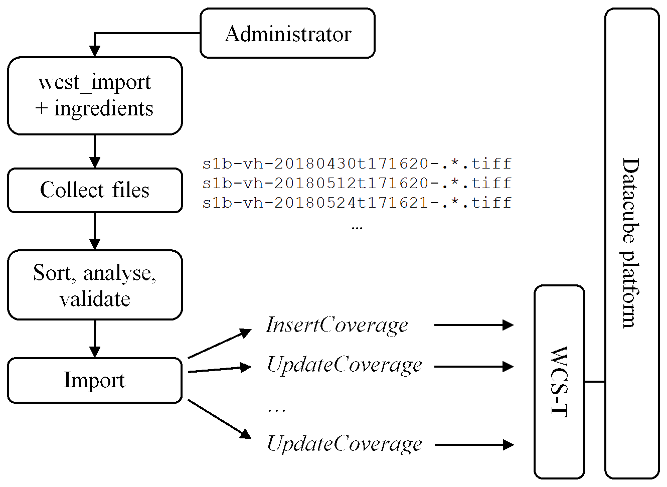
Figure 5.1 Data importing process with wcst_import.sh
An ingredients file showing all possible options (across all recipes) can be found here in the same directory there are several examples of different recipes.
The following recipes are provided in the rasdaman repository:
Specialized recipes
For each one of these there is an ingredients example under the ingredients/ directory, together with an example for the available parameters Further on each recipe type is described in turn, starting with the common options shared by all recipes.
Note
It is required to run only one wcst_import.sh process for registering / importing
files to one specific coverage. Running multiple wcst_import.sh processes
for building multiple different coverages are allowed (the maximum number of processes
is equivalent to the number of rasservers configured in rasmgr.conf file).
5.9.2. Common Options
Some options are commonly applicable to all recipes. We describe these options for each top-level section of an ingredient file: config, input, recipe, and hooks.
5.9.2.1. config section
service_url- The endpoint of the WCS service with the WCS-T extension enabled
service_is_local-trueif the WCS service endpoint runs locally on the same machine,falseotherwise. When set tofalse, the data to be imported will be uploaded to the remote host. This may also be done even when the WCS service endpoint runs locally but has no read permissions on the data files, in which case the only way to import the data is by uploading it to the server; note, however, that this adds a performance penalty, so it should be avoided whenever possible. By default this setting istrue.
mock- Print WCS-T requests but do not execute anything if set totrue. Set tofalseby default.automated- Set totrueto avoid any interaction during the data import process. Useful in production environments for automated deployment for example. By default it isfalse, i.e. user confirmation is needed to execute the actual import.blocking(since v9.8) - Set tofalseto analyze and import each file separately (non-blocking mode). By default blocking is set totrue, i.e. wcst_import will analyze all input files first to create corresponding coverage descriptions, and only then import them. The advantage of non-blocking mode is that the analyzing and importing happens incrementally (in blocking mode the analyzing step can take a long time, e.g. days, before the import can even begin).Note
When importing in non-blocking import mode for coverages with irregular axes, it will only rely on sorted files by filenames and it can fail if these axes’ coefficients are collected from input files’ metadata (e.g: DateTime value in TIFF’s tag or GRIB metadata) as they might not be consecutive. wcst_import will not analyze all files to collect metadata to be sorted by DateTime as in default blocking import mode.
default_null_values- This parameter adds default null values for bands that do not have a null value provided by the file itself. The value for this parameter should be an array containing the desired null value either as a closed intervallow:highor single values. Example:Note
If set this parameter will override the null/nodata values present in the input files and the
nil_valueornil_valuessettings specified in the ingredients file.If this parameter is not set, wcst_import will try to detect these values for bands implicity from the first input file.
If set this parameter to:
[], then, wcst_import will create a coverage without any null values.
Note
If a null value interval is specified, e.g
"9.96921e+35:*", during encode it will not be preserved as-is because null value intervals are not supported by most formats. In this case it is recommended to first specify a non-interval null value, followed by the interval, e.g.[9.96921e+35, "9.96921e+35:*"].tmp_directory- Temporary directory in which gml and data files are created; should be readable and writable by rasdaman, petascope and current user. By default this is/tmp.crs_resolver- The crs resolver to use for generating WCS-T request. By default it is determined from thepetascope.propertiessetting.url_root- In case the files are exposed via a web-server and not locally, you can specify the root file url here; the default value is"file://".
skip- Set totrueto ignore files that failed to analyze (i.e. file can be accessed but it is not possible to open and read its content) or failed to import to rasdaman. If set tofiles_that_fail_to_open, then files that failed to analyze will be skipped, however if a file failed to import to rasdaman, then import process is terminated. By default it isfalse, i.e. the import process is terminated when a file fails to import.retry- Set totrueto retry a failed request. The number of retries is either 5, or the value of settingretriesif specified. This is set tofalseby default.retries- Control how many times to retry a failed WCS-T request; set to 5 by default.retry_sleep- Set number of seconds to wait before retrying after an error; a floating-point number can also be specified for sub-second precision. Default values is 1.track_files- Set totrueto allow input files to be tracked in a JSON file<coverage_id>.resume.jsoncontaining a list of imported file paths, in order to avoid reimporting them when wcst_import.sh is subsequently executed again. The JSON file is generated in the directory set by theresumer_dir_pathsetting. This setting is enabled by default. Example content of a resume fileS2_L2A_32633_B01.resume.jsonof a coverageS2_L2A_32633_B01:resumer_dir_path- The directory in which to store the resume file generated whentrack_filesis set totrue. The user invoking wcst_import.sh must have permissions to write in this directory. By default the resume file will be stored in the same directory as the ingredients file.slice_restriction- Limit the slices that are imported to the ones that fit in a specified bounding box. Each subset in the bounding box should be of form{ "low": 0, "high": <max> }, where low/high are given in the axis format. Example:description_max_no_slices- Maximum number of slices (files) to show for preview before starting the actual data import.subset_correction(deprecated since v9.6) - In some cases the resolution is small enough to affect the precision of the transformation from domain coordinates to grid coordinates. To allow for corrections that will make the import possible, set this parameter totrue.
5.9.2.2. input section
coverage_id- The name of the coverage to be created; if the coverage already exists, it will be updated with the new files collected bypaths.paths- List of absolute or relative (to the ingredients file) paths or regex patterns in format acceptable by the Python glob function. Multiple paths separated by commas can be specified. The collected file paths are by default sorted in ascending order before import, either by calculated datetime in time-series recipes, or by lexicographic comparison of the file path strings otherwise. The ordering can be changed to descending or disabled completely with the import_order option.Note
wcst_import analyzes each input file from
pathsand maximum time to open one file for this purpose is 60 seconds. If during this time the file cannot be opened, then wcst_import will try to open it two more times. If the file is still not possible to open, then it will:throw exception and stop the importing process if
skipsetting isFalse, orignore this file and continue with the other input files if
skipsetting isTrue
inspiresection contains the settings for importing INSPIRE coverage:metadata_url- If set to non-empty string, then the importing coverage will be marked as INSPIRE coverage, see more details here. If set to empty string or omitted, then the coverage will be updated as non-INSPIRE coverage.
5.9.2.3. recipe section
tiling- (required) Specifies the tile structure to be created for the coverage in rasdaman. You can set arbitrary tile sizes for the tiling option only if the tile name isALIGNED. Example:For more information on tiling check Storage Layout Language
import_order- Indicate in which order the input files collected with thepathssetting should be imported. In time-series recipes, the ordering is based on the datetime calculated for each file. In other recipes, e.g.map_mosaic, the ordering is based on lexicographic comparison of the file paths. Possible values are:ascending(default) - import files in ascending order;descending- import files in descending order;none- do not order files in any particular way before import.
Example:
thumbnail_path- Absolute/relative path to a PNG/JPEG file to be associated as a thumbnail of the imported coverage (docs). This setting has an effect only when the coverage does not yet exist. An image size of 250x250 pixels is recommended. Example:"thumbnail_path": "raster_image_resized_to_250x250.png"
wms_import- If set totrue(applicable only when layer does not exist), after importing data to coverage, it will also create a WMS layer from the imported coverage and populate metadata for this layer. After that, this layer will be available from WMS GetCapabilties request. Example:
wms_styles- An array of style definitions to be added to a WMS layer after it was created with"wms_import": true. If not specified no styles are added to the layer. Each style definition is a JSON object of mandatory and further optional properties:name(mandatory) - name identifier of the style composed of alphanumeric characters and_(regular expression pattern[a-zA-Z][a-zA-Z0-9_]*)title(mandatory) - human-readable title of the styleabstract(mandatory) - short human-readable description of the styledefault(optional) - set totrueto set this style as default, i.e. a WMSGetMapwith emptySTYLESrequest parameter will apply this style to the result; by default it is set tofalsewcps_query_fragment(optional) - a WCPS query fragment to define additional query expressions for applying to the result; exclusive withrasql_query_fragmentrasql_query_fragment(optional) - a rasql query fragment to define additional expressions for applying to the result; exclusive withwcps_query_fragmentcolor_map(optional) - a relative/absolute path to a JSON file containing a ColorMap style; exclusive withgdal_color_tableandsld_color_tablegdal_color_table(optional) - a relative/absolute path to a JSON file containing a GDAL color style; exclusive withsld_color_table``and ``color_mapsld_color_table(optional) - a relative/absolute path to an XML file containing an SLD color style; exclusive withgdal_color_tableandcolor_maplegend(optional) - a relative/absolute path to a PNG or JPEG file to be added as the legend graphic of the style
More details can be found on the corresponding API documentation.
Example of adding 6 different styles to a layer:
scale_levels- Enable the WMS pyramids feature. Level must be positive number and greater than 1 (note: only spatial geo axes, e.g. Lat and Long are scaled down in the pyramid member coverage). A new coverage as pyramid member of the importing coverage will be created with this pattern. Syntax:scale_factors- Enable the WMS pyramids feature. It is a more flexible variant of thescale_levelssetting. The two settings are exclusive, eitherscale_levelsorscale_factorscan exist in the ingredient file. The coverage_id of each factor must be unique in rasdaman and manually set by the user. The factors is a list of decimal values corresponding to the coverage axes according to its CRS order; a scale value for an irregular axis must be 1, while for a regular axis it should be greater than 1; see more details here. For example, you can create two pyramid member 2D coverages which are 2x smaller (cov_level_2) and 4x smaller (cov_level_4) on the regular Lat and Long axes:import_overviews- If specified with indices (0-based), wcst_import will import the corresponding overview levels defined in the input files as separated coverages with this naming pattern. The selected overview coverages are then added as pyramid memberds to the base importing coverage. For example, to import overview levels 0 and 3 from a tiff file which has 4 overview levels in totalyou can specify
"import_overviews": [0, 3]in the ingredients.By default this setting is set to an empty array, i.e. no overview levels will be imported. Only GDAL recipes and gdal version 2+ are supported.
import_all_overviews- If specified withtrue, all overview levels which exist in the input files will be imported. For example, to import all 4 overview levels from a tiff file you can specify"import_all_overviews": truein the ingredient file.This setting and
import_overviewsare exclusive, only one can be specified. By default it is set to false. Only GDAL recipes and gdal version 2+ are supported.import_overviews_only- If specified withtrue, input files are not imported to the base coverage specified withcoverage_id, but only to the overview coverages as specified in the ingredients file by eitherimport_all_overviewsorimport_overviews. This setting is set tofalseby default if not specified explicitly.Note
If the input files were already imported to the base coverage and they were tracked in
<base_coverage_id>.resume.json, it is necessary to remove this resume file in order to import only the overview coverages. Alternatively the ingredients file can be copied to another directory and adapted to setimport_overviews_onlytotrue.
pyramid_members- List of existing coverages which can be added as pyramid members of the importing coverage, see request. Syntax:pyramid_bases- List of existing coverages to which the importing coverage will be added as a pyramid member. This parameter has the opposite effect ofpyramid_members, see corresponding request. Syntax:pyramid_harvesting- If set totrue, recursively add all nested pyramid members of the pyramid member coverage to the target base coverage. The pyramid member coverage depends on which of these two settings is used:If
pyramid_basesis specified, then the currently importing coverage is the pyramid member of the the base coverages listed inpyramid_bases;Otherwise, if
pyramid_membersis specified, then the currently importing coverage is the base coverage of the pyramid member coverages listed inpyramid_members;Otherwise, if neither of the above options is specified, an error is throws.
See request for more details on the underlying request sent to petascope when this option is set to
true. By default this option is set tofalse.
5.9.2.3.1. Image pyramids
Since v9.7 it is possible to create downscaled versions of a given coverage, eventually achieving something like an image pyramid, in order to enable faster WMS requests when zooming in/out.
By using the scale_levels option of wcst_import
when importing a coverage with WMS enabled, petascope will create downscaled
collections in rasdaman following this pattern: coverageId_<level>.
If level is a float, then the dot is replaced with an underscore,
as dots are not permitted in a collection name. Some examples:
MyCoverage, level 2 -> MyCoverage_2
MyCoverage, level 2.45 -> MyCoverage_2_45
Example ingredients specification to create two downscaled levels which are 8x and 32x smaller than the original coverage:
Two new WCS-T non-standard requests are utilized by wcst_import for this feature, see here for more information.
5.9.2.4. hooks section
5.9.3. Introduction
When ingesting files with wcst_import, commands can be executed before ingestion/registration starts and after successful ingestion. Behavior is specified in so-called hooks, subdivided into before hooks executed before ingestion and after hooks executed after(successful) ingestion.
Multiple before/after hooks can be specified, and they will be evaluated in the
order in which they are specified. When import mode is set to non-blocking
("blocking": false), wcst_import will run before/after hook(s) for the file
which is being used to update coverage, while the default blocking importing
mode will run the hooks for all input files before/after they are imported
into a coverage.
Technically, these commands get executed in a bash shell forked by the import process. Commands can be parametrized through a series of variables made available through “data expressions”, including the input file name, target coverage, and several more. These are tailored for the specific purpose of working before and after the actual ingestion.
A common use case is that, from the original input file, some intermediate file is derived which subsequently is ingested instead. Further use cases include writing a “successfully done” file, removing the original file, sending a success message, etc.
5.9.4. Syntax
Hooks are specified in a hooks top-level configuration in an ingredient file
(on the same level as the config, input, and recipe sections):
"hooks": [ hook1, hook2, ... ]
Each hook is a JSON object in the "hooks" JSON array, with parameters as
follows:
description(mandatory) - Human-readable description what this ingestion hook does(mandatory); wcst_import prints the description when applying the hook during import.when(mandatory) - Run a command before (before_import) or after (after_import) importing the files into a coverage.cmd(mandatory, exclusive withpython_cmd) - specify Bash commands to be executed with/bin/bashin the current working directory from whichwcst_import.shis invoked. Standard error and output from executing the commands are both redirected to stdout by wcst_import. The Bash code is executed in a Bash process newly forked for every file.Note
If there are many files, using
cmdcan be costly in terms of performance and memory usage and it may be better to usepython_cmd.python_cmd(mandatory, exclusive withcmd) - specify Python code, which is evaluated in the same Python instance already running wcst_import with the exec() method. It may be preferable to Bashcmdwhen there are many files to import, or more complex tasks need to be performed with advance math calculations, for example.Note
As an ingredients file can contain arbitrary Python or Shell code which wcst_import will execute before/after importing files or during the evaluation of sentence expressions, it can pose a security issue if untrusted users are allowed to write ingredients files to be executed with wcst_import. In this case, it is recommended to make sure the user executing wcst_import is properly restricted on their ingredients files.
abort_on_error(optional) - If set totrue, when acmdbash command returns an error or when apython_cmdraises anException, wcst_import terminates immediately. Applicable only ifwhenis set tobefore_import.replace_path(optional) - wcst_import will consider the specified absolute paths (globbing is allowed) as the actual absolute file paths to be imported after running a hook, rather than the original input file paths configured inpathssetting of theinputsection.If there are multiple hooks, the
replace_pathwill be effective in all hooks following the hook where it’s defined. If areplace_pathis specified in one of the following hooks, it will become the current replace_path once that hook gets executed (as they are executed in order).Applicable only if
whenis set tobefore_import.execute_if(optional) - A value ofimport_succeeded(default) indicates that the hook should be executed only for successfully imported files; a value ofimport_failedindicates that the hook will be executed only when a file fails to import for some reason (note that this only works when(“skip”: true) is set, as otherwise the import process will stop before the after hook has a chance to run). Applicable only ifwhenis set toafter_import.
5.9.5. Data expressions
Hooks can make use of data expressions
which are provided for various purposes. Specifically for cmd /
python_cmd, the input file path provided through ${file:path} is
relevant. Prior to command execution these expressions get substituted by their
current value in both before and after hooks.
In addition, the bounding box of the datacube area effectively updated is available, with its value being the same in before and after hooks:
${bbox}: the multi-dimensional bounding box of the data region affected by the update; for each axis there is one element, identified by its axis label (case-sensitive), with two components: *min: the minimum bbox value along this axis *max: the maximum bbox value along this axis
Examples:
${file:path}.aux[ ${bbox:Lat:min} : ${bbox:Long:max} ]${bbox:time:max}
5.9.6. Hook evaluation
On each input file the following three steps are performed:
All before hooks defined in the ingredient file get evaluated in the order in which they are specified;
${file:path}and${bbox}are available. - errors will terminate the import ifabort_on_erroris set totrue.The import process takes place on the file referenced in
${file:path}, unless overriden with thereplace_pathssettingAll after hooks get evaluated in in the order in which they are specified;
${file:path}and${bbox}are available.
5.9.7. Examples
Example: Import GDAL subdatasets
The example ingredients below contains a before hook which replaces the collected file path into a GDAL subdataset form; in this particular case, with the GDAL driver for NetCDF a single variable from the collected NetCDF files is imported.
Example: Preprocess GDAL files before importing
This example ingredients below contains
a
before_importhook which runs a bash command to project each input tiff file to a temp tiff file in EPSG:4326 CRS, which become the actual paths to import.an
after_importhook which removes the temp file paths from the before hook once they have been imported successfully.
5.9.8. Best practices
The following recommendations are not mandatory for rasdaman to work properly, and they are not system-enforced, but they have proven useful in day-to-day datacube management:
In
cmdenclose all references to files in escaped quotes to properly handle cases where file paths contain whitespace (see Bash documentation for details on escaping):"cmd": "gdalwarp ... \"${file:path}\" \"${file:path}.nc\"",
Make sure the partition where auxiliary files are generated contains sufficient free space.
For each coverage/datacube create a dedicated input directory to keep ingestion traffic disentangled (this degree of freedom generally exists only for ingestion, not for registration).
In
cmdonly use${file:path}as data expression. More general data expressions are available as documented, but their use is discouraged as it may have unforeseen impact once python and shell evaluation start interfering (and, actually, the equivalent functionality is available in bash).
5.9.9. Recipe map_mosaic
Well suited for importing a tiled map, not necessarily continuous; it will place all input files given under a single coverage and deal with their position in space. Parameters are explained below.
5.9.10. Recipe time_series_regular
Well suited for importing multiple 2-D slices created at regular intervals of time (e.g sensor data, satelite imagery etc) as 3-D cube with the third axis being a temporal one.
Note
This recipe should be used to update an existing coverage with new data
only in the case when "track_files": "false" and previously imported files
have not been removed. The timestamp for the first input file
is set by the time_start setting, so if old imported files are removed
the timestamp will be set again to time_start when wcst_import is run again
with new files to be imported. The effect is that new input files will
override the existing time slices instead of adding new time slices on top of time axis.
Parameters are explained below:
5.9.11. Recipe time_series_irregular
Well suited for importing multiple 2-D slices created at irregular intervals of time into a 3-D cube with the third axis being a temporal one. There are two types of time parameters in “options”, one needs to be choosed according to the particular use case:
5.9.12. Recipe general_coverage
This is a highly flexible recipe that can handle any kind of data files (be it 2D, 3D or n-D) and model them in coverages of any dimensionality. It does that by allowing users to define their own coverage models with any number of bands and axes and fill the necesary coverage information through the so called ingredient sentences inside the ingredients.
5.9.12.1. Coverage parameters
Using ingredient sentences we can define any coverage model directly in the options of the ingredients file. Each coverage model contains the following parts:
crs- Indicates the crs of the coverage to be constructed. Either a CRS url can be used e.g. http://localhost:8080/rasdaman/def/crs/EPSG/0/4326 or a shorthand notationCRS1<op>CRS2<op>.., where CRS1/CRS2/.. are of the form EPSG/0/4326 or EPSG:4326, and<op>is either@or+. For example, a time/date + spatial compound CRS could beOGC/0/AnsiDate@EPSG/0/4326, orOGC:AnsiDate+EPSG:4326.metadata- A group of options controlling metadata extraction and consolidation; more detailed information follows belowslicer- A group of options controlling the data decoding and placement into the overall datacube; more detailed information follows below.
5.9.12.1.1. metadata section
The metadata section specifies in which format you want the metadata (xml).
It can only contain characters and is limited in size by the backend
database limit for CLOB columns; for postgresql (the default backend for
petascope) the maximum size is 2GB (source).
type- Specifies the format for storing the coverage metadata;xmlis supported, and it is set toxmlby default.
global- Specifies fields which should be saved once as rasdaman metadata (XML prefixras:) for the whole coverage (e.g. title, data licence, creator etc). For example a “Title” metadata value can be set with"global": { "Title": "'Drought code'", ... }.Global metadata will be collected automatically for netCDF and gdal recipe from the first input file, if the
"global"setting is omitted, or it is set to"auto". From netCDF data, the attributes of each variable as well as the global attributes are collected. In case of importing with agdalslicer, the GDAL metadata will be collected.This automatic collection is not done when additional global metadata needs to be added on top of the metadata present in the input file; in this case both the metadata from the file and the additional metadata have to be specified explicitly.
The specified/collected metadata will be listed in the DescribeCoverage rasdaman metadata.
coverage_metadata- An array of strings which are valid XML, which will be added to the coverage metadata visible in a WCSDescribeCoverageresponse. This metadata will be added as siblings of the metadata under the rasdaman namespace defined via theglobalsetting above. Example to addSTACcatalog metadata to a coverage calledLGN:local- Specifies fields which are fetched from each input file to be stored in coverage’s metadata. When subsetting in the output coverage only local metadata associated to the subsetted areas will be added to the result. E.g.,"local": { "LocalMetadataKey": "${netcdf:metadata:LOCAL_METADATA}" }sets LocalMetadataKey to a metadata value extracted from the input data; the${..}is explained in Data expressions. For a more detailed explanation of local metadata see the dedicated Local metadata from input files section.
colorPaletteTable- Controls collection of color palette table for the created coverage, which can then be used internally when encoding coverage to, e.g. PNG, to colorize the result. Currently only GDAL-stylecolorTablewith 256 color entries is supported (GDAL docs <https://gdal.org/user/raster_data_model.html#color-table>).A path to an explicit Color Palette Table
.cptfile can be specified; such a file can be referenced in the ingredients file with, e.g.,"colorPaletteTable": "PATH/TO/table.cpt".If
colorPaletteTableis set to"auto"or not specified at all, and the slicer is set togdal(see next section for info on slicers), then the color table will be read automatically from the first input file if its metadata contains one.If
colorPaletteTableis set to an empty string"", any color table metadata will be ignored when creating coverage’s global metadata.The specified/collected color palette table will be listed in the DescribeCoverage rasdaman metadata.
bandsandaxes- Allow specifying metadata for the coverage bands and/or axes; more details can be found in Band and axis metadata in global metadata.
5.9.12.1.2. slicer section
The slicer subsection specifies the driver to use to read from the data files,
the required bands from data files and for each axis from the CRS how to obtain the
bounds and resolution corresponding to each file.
type- Specifies the decoding driver to be used; currently the following are supported:gdal- for TIFF, PNG, and other encoding format that can be read with GDAL (check withgdalinfo <file>);netcdf- for importing NetCDF data. If a netCDF file is flipped on Lat axis (South -> North coordinates increase in the output ofncdump -c) instead of GDAL style (North -> South coordinates decrease), then it is necessary to flip it before importing as rasdaman, e.g. withcdo invertlat input.nc output.nc.grib- for GRIB data. Currently, rasdaman only supports GRIB files withgridTypeformat of regular lat longregular_ll. If the format is different, it is necessary to preprocess the input files into regular grid type. The grid type can be retreived withgrib_dump file.grib | grep 'gridType'.If a GRIB file is flipped on Lat axis (South -> North with
jScansPositively = 0in the output ofgrib_dump) instead of GDAL style (North -> South withjScansPositively = 1), then it is necessary to flip it before importing to rasdaman, e.g. withcdo invertlat input.grib output.grib.
subtype- Specify a slicer subtype. Currently only"sentinel2"is supported as a value, valid in combination with"type": "gdal". When present in the ingredients, instead of opening files to be imported with GDAL in order to read needed metadata such as CRS and geo bbox, this will be done by reading theMTD_TL.xmlfile present in the SAFE container that contains the file to be imported. This can be much faster compared to reading the metadata from JPEG 2000 files with GDAL. Note that this only works with file paths on the filesystem in extracted SAFE directories, or with SAFE directories on S3 object storage. In the latter case, wcst_import will try to use s3cmd to retrieve theMTD_TL.xmllocally first in/tmp/rasdaman_wcst_import/; these temporary files need to be manually removed.pixel_is_point- Only valid iftypeisnetcdforgrib. In some cases, by convention in the input files, the coordinates are set in the middle of grid pixels, hence, set totrueto extend the lower and upper bounds of each regular axis by half grid pixel to be able to import. By default it is set tofalse.bands- A list of bands/chanels/variables from the input files which should be imported to the importing coverage. Each entry is a JSON object with the following options, of whichidentifierandnameare mandatory to specify while the rest are optional:identifier- The unique name of the band in the input file. With GDAL the band can be integer number (zero-based index). With GRIB data, only one band can be specified in the ingredients file, and the band identifier must match theshortNamefield in the GRIB messsages so only those messages will be imported. If no messages matched the band identifier, then all GRIB messages will be imported; this only works for input GRIB files with only one band.name- The unique name of the band which will be used in the created coverage; this can be different from theindentifier;label- The label of the band according toswe:labelelement; if not set, then, it is set to the name of the band (field’s name)observation_type- set the output type in GML format of a band in SWE standard. If omitted, then it set tonumericalby default. Valid values are:numeric(in GML showed asswe:Quantity) andcategorial(in GML showed asswe:Category).description- Metadata description of the band;definition- Metadata definition of the band, typically it is a URL pointing to online registries, ontologies or dictionaries. If omitted, petascope sets the value to the URL corresponding to band’s data type.nil_value`- Metadata null value of the band; used in case band has only one null value.If
default_null_valuessetting is specified, thennil_valuesetting is ignored.nil_reason- Metadata reason for the null value of the band;uom_code- Set the Unit of measurement (uom) code of the band. Besides setting it directly, it can also be derived from the input file metadata, with e.g.${netcdf:variable:NAME:units}for NetCDF or${grib:unitsOfFirstFixedSurface}for GRIB. Note: only valid forswe:Quantity.code_space- List and define the meaning of all possible values for this component. Note: only valid forswe:Category.${grib:unitsOfFirstFixedSurface}for GRIB. Note: only used forswe:Category.filter_messages_matching- Default is empty. If not-empty (a dictionary of user input GRIB keys:values; keys (e.g.shortName) must exist in the input GRIB files), then it filters any GRIB message which has a GRIB value not contain a user input value of a GRIB key.Further
"key": "value"entries can be specified to add customized band metadata to the global coverage metadata.
axes- A JSON object which configures the properties of each axis of the created coverage with"axisLabel": { properties... }. The possible properties are listed below; generally,grid_order,min,max, andresolutionhave to be specified, except for irregular axes whereresolutionis not applicable.grid_order- specify the grid order of axes defined by the coverage CRS. If not specified, wcst_import will try to automatically derive the grid_order according to the documentation below. That may fail with unusual data, in which case it will be necessary to set this setting manually for each axis.Axes of a CRS which is not part of the file CRS have grid_order that is same as the order in the CRS definition. For example, if the coverage CRS is a compound CRS
OGC/0/AnsiDate@EPSG/0/4326and data files themselves have CRSEPSG/0/4326, then grid_order for the ansi axis inOGC/0/AnsiDatewill be 0, and the grid_order of theEPSG/0/4326axes will follow with 1 and 2. If the CRS order was reversed toEPSG/0/4326@OGC/0/AnsiDate, then the grid_order of 4326 axes (Long/Lat) would be 0 and 1, and of AnsiDate (ansi) would be 2. Usually axes of non-file CRS (AnsiDate in this example) will also have settingdata_bound: false.Below we give hints on how to determine the grid_order of axes in the file CRS.
When data is imported with the
gdalorgribslicer, generally the grid_order isnfor X axes (Longitude, E, …), andn+1for Y axes (Latitude, N, …).When importing data with the
netcdfslicer, the grid_order should usually match the dimension order of the imported variable, which can be checked withncdump -h; e.g. a variablefloat dc(time, lat, lon)will have grid_ordernfor time,n+1for lat, andn+2for lon. This will work well as long as the data conforms to the CF-conventions <https://cfconventions.org/Data/cf-conventions/cf-conventions-1.7/cf-conventions.html#dimensions>, and may otherwise need adjustments if the spatial dimensions are not in Y/X order.
crs_order- The index of the geo axis in the coverage’s CRS (0-based). Note: By default it is not required. Only set when one specifies a different name for this axis, than the one configured in the CRS’s definition; more details can be found here; In this case, each axis must have an unique indexcrs_orderspecified.min- The lower bound of the axis (coordinates in the axis CRS);max- The upper bound of the axis (coordinates in the axis CRS);resolution- The resolution of the axis from the input file; if this axis is irregular, the resolution is set to1;statements- Import python utility libraries (e.g.datetime/timedelta) to support calculatingmin,max,resolution, etc; covered in more detail in a subsequent section;
A few additional options are specific to irregular axes:
irregular- Set totrueto specify that this axis is irregular, e.g. a time axis with irregular datetime indexes; if not specified, it is set tofalseby default;direct_positions- A list of coefficients which are extracted and calculated based on the axis lower bound from the irregular axis values specified in the input netCDF/GRIB file.For example, let’s consider a netCDF file that has a
timedimension with attributeunits: "days since 1970-01-01 00:00:00". All stored values of thetimeaxis must be converted to datetime based on the lower bound value ("1970-01-01") as an origin.data_bound- Set tofalseto specify that this axis should be imported as a slicing point instead of a subset with lower and upper bounds; typical use case for this is when extracting irregular datetime values from the input file names. When not specified it is set totrueby default.For example, the indexes of an irregular axis
ansicould be extracted from dates in the file names of input netCDF files (e.g.GlobLAI-20030101-20030110-H01V06-1.0_MERIS-FR-LAI-HA.nc) through a regular expression.slice_group_size- Group multiple input slices into a single slice in the created coverage, e.g., multiple daily data files onto a single week index on the coverage time axis; explained in more detail here;
areas_of_validity- Specify a list ofstartandendbounds for each coefficient in an irregular axis to extend their areas to[start, end]intervals (see Areas of validity on irregular axes). The start/end intervals must not overlap, and the number of pairs must equal the number of coefficients imported.The start and end may be specified with less than millisecond precision, e.g.
"2010"and"2012-05". In this case they are expanded to millisecond precision internally such that start is the earliest possible datetime starting with"2010"(i.e."2010-01-01T00:00:00.000Z") and end is the latest possible datetime starting with"2012-05"(i.e."2012-05-31T23:59:59.999Z"). The same semantics applies in subsetting in queries, see Temporal subsets.By default if not specified, a coefficient is a single point.
The example below imports 3 input files with the datetime coefficients for the irregular axis
ansicollected from the filename ("data_bound": false) and custom areas of validity for the 3 coefficients:
validity- Specify areas of validity for each coefficient of the current irregular axis. This setting is exclusive with theareas_of_validitysetting. The following options can be specified:"type"- (required) currently the only valid value isnext_slice. First the area of validity of the coefficientCof the file currently being imported is initialized to[C, C]. This can be adjusted with the"start"and"end"options below.Second, the file is imported at a coefficient
Pin the datacube in rasdaman. If the datacube is empty, i.e. no coefficients exist yet, then the coefficient and its area of validity are inserted as calculated in the the first step. IfPalready exists in the datacube, then its area of validity remains unchanged. If a coefficient precedingPexists, then the upper bound of its area of validity is set toC - 1ms(1 millisecond less than the lower bound of the input file’s area of validity).For example, if an axis time has upper bound
"2015-01-01", and an input slice with with a coefficient"2018-01-01"is being imported, then the area of validity of the"2018-01-01"slice is set to["2018-01-01","2018-01-01"]and inserted in rasdaman, while the area of validity of the"2015-01-01"slice is updated to["2015-01-01", "2017-12-31T23:59:59.999"](one millisecond less than"2018-01-01")."start"- (optional) extend the lower bound of the area of validity of the coefficient of the file currently being imported by the specified duration. Durations start with thePcharacter, e.g.P-1Ydecreases the lower bound by 1 year."end"- (optional) extend the upper bound of the area of validity of the coefficient of the file currently being imported by the specified duration. The format is same as for the"start"option, e.g.P1Yincreases the upper bound by 1 year.
The example below imports input files with the datetime coefficients for the irregular axis
timecollected from the filename ("data_bound": false) and each file’sareas_of_validitywill be adjusted impliticly in petascope when importing new coverage slice:
5.9.12.1.3. Examples
The examples below illustrate importing data in different formats with the
general_coverage recipe.
Commented example for importing GRIB data (only the
recipesection is shown for brevity):
Example for importing NetCDF data as a 3d coverage with an irregular time axis:
Example for importing 2d TIFF files to a 3d coverage with the
gdaldriver
5.9.12.2. Ingredient sentences
An ingredient sentence can be of multiple types:
Numeric - e.g.
2,4.5Strings - e.g.
'Some information'Functions - e.g.
datetime('2012-01-01', 'YYYY-mm-dd')Data expressions - Allow to collect information from the data file being imported with a specific format driver. An expression is of form
${driverName:driverOperation}- e.g.${gdal:minX}or${netcdf:variable:time:min. All possible expressions are documented in Data expressions.Python expressions - The types above can be combined into any valid Python expression; this allows to do mathematical operations, string parsing, date/time manipulation, etc. E.g.
${gdal:minX} + 1/2 * ${gdal:resolutionX}ordatetime(${netcdf:variable:time:min} * 24 * 3600). Expressions can use functions from any Python library which just needs to be explicitly imported as explained in Using libraries in sentences.
5.9.12.3. Data expressions
Each driver allows expressions to extract information from input files.
We will mark with capital letters things that vary in the expression.
E.g. ${gdal:metadata:EXPRESSION} means that you can replace
EXPRESSION with either any valid gdal metadata tag such as TIFFTAG_DATETIME
or bandINDEX:TAGNAME with INDEX is 0-based to get value of specified TAGNAME
of the selected band i-th.
Example ingredients where data expressions are used can be found in Examples.
5.9.12.3.1. NetCDF
Type |
Description |
Examples |
|---|---|---|
Metadata information |
|
|
Variable information |
|
|
Dimension information |
|
|
5.9.12.3.2. GDAL
Relevant for TIFF, PNG, JPEG, and other 2D data formats.
Type |
Description |
Examples |
|---|---|---|
Metadata information |
|
|
Geo Bounds |
|
|
Geo Resolution |
|
|
Origin |
|
|
5.9.12.3.3. GRIB
Type |
Description |
Examples |
|---|---|---|
GRIB Key |
|
|
5.9.12.3.4. File
Type |
Description |
Examples |
|---|---|---|
File Information |
|
|
Imported File Information |
|
|
5.9.12.3.5. BBox
Type |
Description |
Examples |
|---|---|---|
Coverage axis information |
|
|
5.9.12.3.6. Special functions
A couple of special functions are available to help with more complicated expressions:
Function and Arguments |
Description |
Examples |
|---|---|---|
|
This function helps to deal with the usual grib date and time format. It returns back a datetime string in ISO format. |
grib_datetime(${grib:dataDate},
              ${grib:dataTime})
|
|
This function helps to deal with strange date time formats. It returns back a datetime string in ISO format. |
datetime("20120101:1200",
         "YYYYMMDD:HHmm")
|
|
This function extracts information from a string using regex; input is the string you parse, regex is the regular expression, group is the regex group you want to select |
datetime(
  regex_extract('${file:name}',
    '(.*)_(\\d*-\\d\\d)(.*)', 2),
  'YYYY-MM')
|
|
Replaces all occurrences of a substring with another substring in the input string |
replace('${file:path}',
        '.tiff', '.xml')
|
5.9.12.4. Using libraries in sentences
In case the ingredient sentences require functionality from extra Python
libraries, they can be imported with a statements option. For example, to
calculate the lower bound and upper bound for the time axis ansi (starting
days from 1978-12-31T12:00:00) one could use datetime and timedelta
from the datatime library.
Python functions imported in this way override the special functions provided by wcst_import. For
example, the special utility function datetime(date_time_string, format) to
convert a string of datetime to an ISO date time format will be overridden when
the datetime module is imported with a statements setting.
Note
See details about potential issue for running python code in the ingredients file.
5.9.12.5. Local metadata from input files
Beside the global metadata of a coverage, you can add local metadata for each file which is a part of the whole coverage (e.g. a 3D time-series coverage mosaiced from 2D GeoTiff files).
Under the metadata section add a “local” object with keys and values extracted by using format type expression. Example of extracting an attribute from a netCDF input file:
Each file’s envelope (geo domain) and its local metadata will be added to the
coverage metadata under <slice>...</slice> element if coverage metadata is
imported in XML format. Example of a coverage containing local metadata in XML
from 2 netCDF files:
Since v10.0, local metadata for input files can be also fetched from
corresponding external text files with the optional metadata_file option.
For example:
When subsetting a coverage which contains a local metadata section from input files (via WC(P)S requests), if the geo domains of subsetted coverage intersect with some input files’ envelopes, only local metadata of these files will be added to the output coverage metadata.
For example: a GetCoverage request with a trim such that
crs axis subsets are within netCDF file 1:
The coverage’s metadata result will contain local metadata only from netCDF file 1:
5.9.12.6. Customized axis labels
By default, the axes to be configured must be matched by their name as defined
by the coverage CRS. For example, a CRS OGC/0/AnsiDate@EPSG:4326 defines three
axes with labels ansi, Long, and Lat. To configure them, we would have a
section as bellow:
Since v9.8, one can change the default axis label defined by the CRS through
indicating the axis index in the CRS (0-based) with the "crs_order" setting.
For example, to change the axis labels to MyDateTimeAxis, MyLatAxis, and
MyLongAxis:
5.9.12.7. Group coverage slices
Since v9.8, wcst_import allows to group input files on irregular axes (with
"data_bound": false) through the slice_group_size option, which would
specify the group size as a positive number. E.g:
If each input slice corresponds to index X, and one wants to have slice
groups of size N, then the index would be translated with this option to
X - (X % N).
Typical use case is importing 3D coverage from 2D satellite imagery where the
time axis is irregular and its values are fetched from input files by regex
expression. Then, all input files which belong to the same time window (e.g 7
days in AnsiDate CRS with "slice_group_size": 7) will have the same value,
which is the first date of the week.
5.9.12.8. Band and axis metadata in global metadata
Metadata can be manually specified for each band and axis in the ingredient file or automatically derived from input netCDF files. All collected metadata becomes available in the DescribeCoverage rasdaman metadata.
5.9.12.8.1. band metadata
If "bands" is set to "auto" or does not exist under "metadata" in
the ingredient file, all user-specified bands will have metadata which is
collected directly from the corresponding variable attributes in the netCDF
file; this only works with netcdf
slicer.
Otherwise, the user could specify metadata explicitly with keys/value pairs. The band name (e.g. “red”) refers to the rasdaman band name, and not the identifier in the input file. Example:
Note
If no metadata should be automatically collected, nor explicitly specified, it is necessary to explicitly set empty metadata:
"metadata": {
  "type": "xml",
  "bands": {
    "red": {},
    "green": {}
  }
}
5.9.12.8.2. axis metadata
If "axes" is set to "auto" or does not exist under "metadata"
in the ingredient file, all user-specified axes will have metadata which is
fetched directly from the netCDF file. Metadata for one axis is
collected automatically if 1) the axis is not specified, 2) the axis is set
to "auto", or 3) the axis is set to ${netcdf:variable:Name:metadata}.
The axis label for variable is detected from the min or max value
of CRS axis configuration under "slicer/axes" section. For example:
Otherwise, the user could specify metadata explicitly as a dictionary of keys/values. The axis name are the rasdaman CRS axis names, and not the dimension variable names in input files.
Note
If no metadata should be automatically collected, nor explicitly specified, it is necessary to explicitly set empty metadata:
"metadata": {
  "type": "xml",
  "axes": {
    "i": {},
    "j": {}
  }
}
5.9.12.9. Rotated CRS support
If rasdaman is compiled with GDAL v3.4.1+, importing and querying data with rotated CRS COSMO:101 is supported. The netCDF data usually has to be preprocessed before import:
Invert the latitude axis when it is south to north order (lower to upper coordinates):
cdo invertlat input.nc inverted_input.nc
Swap the order of the rotated latitude (rlat) and rotated longitude (rlon) axes when the data variable has rlat,rlon order. For example, the
float CAPE_ML(time, rlat, rlon)variable can be transformed tofloat CAPE_ML(time, rlon, rlat)with the following command:ncpdq --rdr=time,rlon,rlat inverted_input.nc correct_lon_lat.nc
Example ingredient file for importing the CAPE_ML variable from preprocessed COSMO netCDF data:
wcst_import automatically checks if the specified band variables
(CAPE_ML in the above example) have a grid_mapping metadata
entry (e.g. CAPE_ML:grid_mapping = "rotated_pole"), and adds
all metadata from the grid mapping variable (rotated_pole) to
the global metadata of the imported coverage.
With the added grid_mapping section, the global metadata of
the coverage might look as below, for example:
When encoding to netCDF in WCS or WCPS requests with the same
COSMO:101 CRS, rasdaman will add this grid mapping metadata
as a non-dimension variable in the output, so that it has the correct
CRS information. The name of the non-dimension variable in the output
is set from the identifier value (rotated_pole above).
5.9.13. Recipe wcs_extract
Allows to import a coverage from a remote petascope endpoint into the local petascope. Parameters are explained below.
5.9.14. Recipe sentinel1
This is a convenience recipe for importing Sentinel 1 data in particular; currently only GRD/SLC product types are supported, and only geo-referenced tiff files. Below is an example:
The recipe extends general_coverage so
the "recipe" section has the same structure. However, a lot of information
is automatically filled in by the recipe now, so the ingredients file is much
simpler as the example above shows.
The other obvious difference is that the "coverage_id" is templated with
several variables enclosed in ${ and } which are automatically replaced
to generate the actual coverage name during import:
modebeam- the mode beam of input files, e.g.IW/EW.polarisation- single polarisation of input files, e.g:HH/HV/VV/VH
If the files collected by "paths" are varying in any of these parameters,
the corresponding variables must appear somewhere in the "coverage_id"
(as for each combination a separate coverage will be constructed). Otherwise,
the data import will either fail or result in invalid coverages. E.g. if all
data’s mode beam is IW, but still different polarisations, the
"coverage_id" could be "MyCoverage_${polarisation}";
In addition, the data to be imported can be optionally filtered with the
following options in the "input" section:
modebeams- specify a subset of mode beams to import from the data, e.g. only theIWmode beam; if not specified, data of all supported mode beams will be ingested.polarisations- specify a subset of polarisations to import, e.g. only theHHpolarisation; if not specified, data of all supported polarisations will be imported.
Limitations:
Only GRD/SLC products are supported.
Data must be geo-referenced.
Filenames are assumed to be of the format:
s1[ab]-(.*?)-grd(.?)-(.*?)-(.*?)-(.*?)-(.*?)-(.*?)-(.*?).tiffors1[ab]-(.*?)-slc(.?)-(.*?)-(.*?)-(.*?)-(.*?)-(.*?)-(.*?).tiff.
5.9.15. Recipe sentinel2
This is a convenience recipe for importing Sentinel 2 data in particular. It relies on support for Sentinel 2 in more recent GDAL versions. Importing zipped Sentinel 2 is also possible and automatically handled.
Below is an example:
The recipe extends general_coverage so
the "recipe" section has the same structure. However, a lot of information
is automatically filled in by the recipe now, so the ingredients file is much
simpler as the example above shows.
The other obvious difference is that the "coverage_id" is templated with
several variables enclosed in ${ and } which are automatically replaced
to generate the actual coverage name during import:
crsCode- the CRS EPSG code of the imported files, e.g.32757for WGS 84 / UTM zone 57S.resolution- Sentinel 2 products bundle several subdatasets of different resolutions:10m- bands B4, B3, B2, and B8 (base type unsigned short)20m- bands B5, B6, B7, B8A, B11, and B12 (base type unsigned short)60m- bands B1, B8, and B10 (base type unsigned short)TCI- True Color Image (red, green, blue char bands); also 10m as it is derived from the B2, B3, and B4 10m bands.
level-L1CorL2A
If the files collected by "paths" are varying in any of these parameters,
the corresponding variables must appear somewhere in the "coverage_id" (as
for each combination a separate coverage will be constructed). Otherwise, the
import will either fail or result in invalid coverages. E.g. if all data is
level L1C with CRS 32757, but still different resolutions, the
"coverage_id" could be "MyCoverage_${resolution}"; the other variables
can still be specified though, so "MyCoverage_${resolution}_${crsCode}" is
valid as well.
In addition, the data to be imported can be optionally filtered with the
following options in the "input" section:
resolutions- specify a subset of resolutions to import from the data, e.g. only the “10m” subdataset; if not specified, data of all supported resolutions will be ingested.levels- specify a subset of levels to import, so that files of other levels will be fully skipped; if not specified, data of all supported levels will be ingested.crss- specify a list of CRSs (EPSG codes as strings) to import; if not specified or empty, data of any CRS will be imported.
5.9.16. Creating your own recipe
The recipes above cover a frequent but limited subset of what is possible to model using a coverage. WCSTImport allows to define your own recipes in order to fill these gaps. In this tutorial we will create a recipe that can construct a 3D coverage from 2D georeferenced files. The 2D files that we want to target have all the same CRS and cover the same geographic area. The time information that we want to retrieve is stored in each file in a GDAL readable tag. The tag name and time format differ from dataset to dataset so we want to take this information as an option to the recipe. We would also want to be flexible with the time crs that we require so we will add this option as well.
Based on this usecase, the following ingredient file seems to fulfill our need:
To create a new recipe start by creating a new folder in the recipes folder.
Let’s call our recipe my_custom_recipe:
The last command is needed to tell python that this folder is containing python
sources, if you forget to add it, your recipe will not be automatically
detected. Let’s first create an example of our ingredients file so we get a
feeling for what we will be dealing with in the recipe. Our recipe will just
request from the user two parameters Let’s now create our recipe, by creating a
file called recipe.py
Use your favorite editor or IDE to work on the recipe (there are type annotations for most WCSTImport classes so an IDE like PyCharm would give out of the box completion support). First, let’s add the skeleton of the recipe (note that in this tutorial, we will omit the import section of the files (your IDE will help you auto import them)):
The first thing you need to do is to make sure the get_name() method returns
the name of your recipe. This name will be used to determine if an ingredient file
should be processed by your recipe. Next, you will need to focus on the
constructor. Let’s examine it. We get a single parameter called session which
contains all the information collected from the user plus a couple more useful
things. You can check all the available methods of the class in the session.py
file, for now we will just save the options provided by the user that are
available in session.get_recipe() in a class attribute.
In the validate() method, you will validate the options for the recipe
provided by the user. It’s generally a good idea to call the super method to
validate some of the general things like the WCST Service availability and so on
although it is not mandatory. We also want to validate our custom recipe options
here. This is how the recipe looks like now:
Now that our recipe can validate the recipe options, let’s move to the
describe() method. This method allows you to let your users know any
relevant information about the data import before it actually starts. The
irregular_timeseries recipe prints the timestamp for the first couple of
slices for the user to check if they are correct. Similar behaviour should be
done based on what your recipe has to do.
Next, we should define the import behaviour. The framework does not make any
assumptions about how the correct method of data import is, however it offers a
lot of utility functionality that help you do it in a more standardized way. We
will continue this tutorial by describing how to take advantage of this
functionality, however, note that this is not required for the recipe to work.
The first thing that you need to do is to define an importer object. This
importer object, takes a coverage object and imports it using WCST requests. The
object has two public methods, ingest(), which imports the coverage into the
WCS-T service (note: this can be an insert operation when the coverage was not
defined, or update if the coverage exists. The importer will handle both cases
for you, so you don’t have to worry if the coverage already exists.) and
get_progress() which returns a tuple containing the number of imported slices and
the total number of slices. After adding the importer, the code should look like
this:
In order to build the importer, we need to create a coverage object. Let’s see how we can do that. The coverage constructor requires a
coverage_id: the id of the coverageslices: a list of slices that compose the coverage. Each slice defines the position in the coverage and the data that should be defined at the specified positionrange_fields: the range fields for the coveragecrs: the crs of the coveragepixel_data_type: the type of the pixel in gdal format, e.g. Byte, Float32 etc
The coverage object can be built in many ways, we will present one such method. Let’s start from the crs of the coverage. For our recipe, we want a 3D crs, composed of the CRS of the 2D images and a time CRS as indicated. The following lines of code give us exactly this:
Let’s also get the range fields for this coverage. We can extract them again from the 2D image using a helper class that can use GDAL to get the relevant information:
Let’s also get the pixel base type, again using the gdal helper:
pixel_type = gdal_dataset.get_band_gdal_type()
Let’s see what we have so far:
As you can notice, the only thing left to do is to implement the _get_slices() method. To do so we need to iterate over all the input files and create a slice for each. Here’s an example on how we could do that
And we are done we now have a valid coverage object. The last thing needed is to define the status method. This method need to provide a status update to the framework in order to display it to the user. We need to return the number of finished work items and the number of total work items. In our case we can measure this in terms of slices and the importer can already provide this for us. So all we need to do is the following:
We now have a functional recipe. You can try the ingredients file against it and see how it works.
5.9.17. Importing many files
When an ingredient contains many paths to be imported, usually more than 1000, this may lead to hitting some system limits during the import.
In particular when data is imported with the GDAL driver, wcst_import has a
cache of open GDAL datasets to avoid reopening files, which is costly. With
too many open GDAL datasets limit on max open files can be reached, which
is often 1024 (see ulimit -n). wcst_import handles this case by clearing
its cache; however, this may degrade import performance, so increasing the
limit on open files should be considered.
Furthermore, limits on maximum number of threads may be reached as well,
as each open GDAL dataset creates several threads. This will lead to
errors such as fork: retry: Resource temporarily unavailable.
The maximum allowed number can be observed with
cat /sys/fs/cgroup/pids/user.slice/user-<id>.slice/pids.max, where
<id> can be found with id -u <user> for the user with which
wcst_import is executed. Increasing to a larger value, e.g. 4194304,
should solve this issue.
Finally, wcst_import.sh allows to control the gdal cache size with the
-c, --gdal-cache-size <size> option. The
specified value can be one of: -1 (no limit, cache all files),
0 (fully disable caching), N (clear the cache whenever it has
more than N datasets, N should be greater than 0). The
default value is -1 if this option is not specified.
5.10. Data export
WCS formats are requested via the format KVP key (<gml:format>
elements for XML POST requests), and take a valid MIME type as value. Output
encoding is passed on to the the GDAL library, so the limitations on output
formats are devised accordingly by the supported raster formats of GDAL. The valid MIME types which
Petascope may support can be checked from the WCS 2.0.1 GetCapabilities
response:
In case of encode processing expressions, besides MIME types WCPS (and rasql) can also accept GDAL format identifiers or other commonly-used format abbreviations like “CSV” for Comma-Separated-Values for instance.
5.10.1. Support for time in netCDF output
If the global metadata of a coverage contains "units" and "calendar"
settings for the time axis, when encoding to netCDF rasdaman will
adjust the coordinates of the time variable based on the origin specified
in the "units" and "calendar" setting instead of the time CRS.
Only standard and proleptic_gregorian calendars are currently
supported. More details on these standard attributes of time variables
can be found in the CF conventions docs.
For example, a coverage might have this metadata for the ansi
time axis:
The values of ansi variable in the output netCDF file will be
based on the origin 2016-12-01 00:00:00 as specified by the
<units> above, instead of 1600-12-31, the origin of the
AnsiDate CRS associated with this axis.
5.11. rasdaman / petascope Geo Service Administration
The petascope conpoment, which geo services contact through its OGC APIs, uses rasdaman for storing the raster arrays; geo-related data parts (such as geo-referencing), as per coverage standard, are maintained by petascope itself.
Petascope is implemented as a war file of Java servlets. Internally, incoming requests requiring coverage evaluation are translated by petascope, with the help of the coverage metadata, into rasql queries executed by rasdaman as the central workhorse. Results returned from rasdaman are forwarded by petascope to the client.
Note
rasdaman can maintain arrays not visible via petascope (such as non-geo objects like human brain images). Data need to be imported via Data Import, not rasql, for being visible as coverages.
For further internal documentation on petascope see Petascope Developer’s Documentation.
5.11.1. Service Startup and Shutdown
Depending of how java_server is configured in petascope.properties,
starting the petascope Web application is different as follows:
If set to
external, then managing the petascope Web application is done via the system Tomcat in which it is deployed, e.g.$ systemctl start tomcat $ systemctl stop tomcat $ systemctl restart tomcat
If set to embedded then petascope is managed along with rasdaman; see this section for more details.
5.11.2. Configuration
The rasdaman-geo frontend (petascope) can be configured via changing settings in
/opt/rasdaman/etc/petascope.properties.
The settings are listed as key=value pairs per line.
Lines starting with a # are comments and ignored.
If a setting key occurs multiple times, then only the last occurrence is considered
(previous key/value pairs are ignored).
For any changes in this file to take effect in petascope, the system Tomcat
(if deployment is external) or rasdaman
(if deployment is embedded) needs
to be restarted.
5.11.2.1. Database
spring.datasource.urlset the connectivity string to the database administered by rasdaman-geo. Supported databases are PostgreSQL, H2, HSQLDB; for more details, see this section.Default:
jdbc:postgresql://localhost:5432/petascopedbNeed to change: YES when DMBS other than PostgreSQL is used
spring.datasource.usernameset the username for connecting to the above database.Default:
petauserNeed to change: YES when changed in the above database
spring.datasource.passwordset the password for the user specified byspring.datasource.username.Default:
randomly generated passwordNeed to change: YES when changed in the above database
spring.datasource.jdbc_jar_pathabsolute path to the JDBC jar file for connecting to the database configured in settingspring.datasource.url. If left empty, the default PostgreSQL JDBC driver will be used. To use a different DBMS (e.g. H2) download the corresponding JDBC driver, and set the path to it.Default: empty
Need to change: YES when a DMBS other than PostgreSQL is used
spring.datasource.tomcat.initial-sizeset the initial size for JDBC connections in pool.Default:
30 connectionsNeed to change: NO
spring.datasource.tomcat.max-activeset the maximum number of active JDBC connections in pool.Default:
70 connectionsNeed to change: NO
spring.datasource.tomcat.max-idleset the maximum number of idle JDBC connections in pool.Default:
30 connectionsNeed to change: NO
metadata_urlset the connectivity string to the database administered by rasdaman-geo. This setting is only used for database migration from one DBMS to another (e.g. PostgreSQL to H2) with migrate_petascopedb.sh; in this casemetadata_urlis used to connect to the source database, whilespring.datasource.urlis used to connect to the target database.Default:
jdbc:postgresql://localhost:5432/petascopedbNeed to change: YES when migrating from a DMBS different from PostgreSQL
metadata_userset the username for the above databaseDefault:
petauserNeed to change: YES when different in the above database
metadata_passset the password for the user specified bymetadata_userDefault:
petapasswdNeed to change: YES when different in the above database
metadata_jdbc_jar_pathabsolute path to the JDBC jar file for connecting to the database configured in settingmetadata_url. If left empty, the default PostgreSQL JDBC driver will be used. To use a different DBMS (e.g. H2) download the corresponding JDBC driver, and set the path to it.Default: empty
Need to change: YES when a DMBS other than PostgreSQL is used
5.11.2.2. General
server.contextPathwhen rasdaman-geo is running in embedded mode (setting java_server), this setting allows to control the prefix in the deployed web application URL, e.g. the/rasdamaninhttp://localhost:8080/rasdaman/ows.Default:
/rasdamanNeed to change: NO
secore_urlsset SECORE endpoints to be used by rasdaman-geo. Multiple endpoints for fail-safety can be specified as a comma-separated list, attempted in order as listed. By default,internalindicates that rasdaman-geo should use its ownSECORE, which is more efficient as it avoids external HTTP requests.Default:
internalNeed to change: NO
Note
If none of the configured resolvers work as expected, then a default CRS resolver endpoint
http://crs.rasdaman.com/defwill be used.crs_domainset the domain to be used for CRS URLs in results of WCS GetCapabilities / DescribeCoverage / GetCoverage requests.Default:
https://opengis.net/defNeed to change: NO
xml_validationif set totrue, WCSPOST/SOAPXML requests will be validated againstOGC WCS 2.0.1schema definitions; when starting Petascope it will take around 1-2 minutes to load the schemas from the OGC server.Note
Passing the OGC CITE tests requires this parameter to be set to
false.Default:
falseNeed to change: NO
ogc_cite_output_optimizationiftrue, rasdaman-geo will optimize responses in order to pass a couple of invalid OGC CITE test cases. Indentation ofWCS GetCoverageandWCS DescribeCoverageresults, for example, will be trimmed.Note
If
true, then it also changes subsetting behavior to allow to slice at axis bound in the cases below:subset_min = axis_maxifaxis_res > 0subset_min = axis_minifaxis_res < 0
Default:
falseNeed to change: NO, except when executing OGC CITE tests
petascope_servlet_urlset the service endpoint in<ows:HTTP>elements of the result ofGetCapabilities. Change to your public service URL if rasdaman-geo runs behind a proxy; if not set then it will be automatically derived, usually tohttp://localhost:8080/rasdaman/ows.Default: empty
Need to change: YES when rasdaman-geo runs behind a proxy.
max_wms_cache_sizeset the maximum amount of memory (in bytes) to use for caching WMSGetMaprequests. This setting speeds up repeating WMS operaions over similar area/zoom level. It is recommended to consider increasing the parameter if the system has more RAM, but make sure to correspondingly update the-Xmxoption for Tomcat as well. The cache evicts least recently inserted data when it reaches the maximum limit specified here.Default:
100000000(100 MB)Need to change: NO
uploaded_files_dir_tmpset an absolute path to a server directory where files uploaded to rasdaman-geo by a request will be temporarily stored; the user running rasdaman-geo (either tomcat or rasdaman) should have write permissions on the specified directory.Default:
/tmp/rasdaman_petascope/uploadNeed to change: NO
full_stacktraceslog only stacktraces generated by rasdaman (false), or full stacktraces including all external libraries (true). It is recommended to keep this setting tofalsefor shorter exception stacktraces inpetascope.log.Default:
falseNeed to change: NO
inspire_common_urlset the URL to an external catalog service for the INSPIRE standard, to be provided by the user. If not set then it will be automatically derived from the petascope_servlet_url setting.Default: empty
Need to change: NO
inspire_dls_spatial_dataset_identifierset the identifier for INSPIRE service name to make WCS GetCapabilities INSPIRE-compliant. If not set then it israsdamanby default.Default: empty
Need to change: NO
batch_job_result_dirsset directories with a limit size specified after the path owned by system user running petascope. For example:batch_job_result_dirs=/data/jobs,limit=10GB;/data2/jobs,limit=20GB. If not specified, then petascope will store output files from finished batch jobs to/tmp/rasdaman_petascope/openeo,limit=100GB.Default: empty
Need to change: NO
batch_job_expirationset seconds from current time to mark finished batch jobs as expired. If a batch job expires, then its output file is removed from server to save space for new jobs.Default: 3600
Need to change: NO
5.11.2.3. Deployment
java_serverspecify how is rasdaman-geo deployed:embeddedstarts the Web application standalone with embedded Tomcat, listening on theserver.portsetting as configured below, whileexternalindicates thatrasdaman.waris deployed in thewebappsdir of external Tomcat.It is recommended to set
embedded, as there is no dependency on external Tomcat server,petascope.logcan be found in the rasdaman log directory/opt/rasdaman/log, and start/stop of rasdaman-geo is in sync with starting/stopping the rasdaman service. Setting toexternalon the other hand can be preferred when there is already an existing Tomcat server running other Web applications.Default:
embeddedNeed to change: NO, unless rasdaman-geo is deployed in external Tomcat
Note
petascope is currently incompatible with Tomcat 10.0 or later. If deploying in an external Tomcat, at most Tomcat 9 must be installed. On Ubuntu 24.04 and later this requires custom installation of Tomcat, as only the
tomcat10package is available by default.server.portset the port on whichembeddedrasdaman-geo (java_server=embeddedabove) will listen when rasdaman starts. This setting has no effect whenjava_server=external.Default:
8080Need to change: YES when port
8080is occupied by another process, e.g. external Tomcat
static_html_dir_pathabsolute path to a directory containing static demo Web pages (html/css/javascript). If set, rasdaman-geo will serve theindex.htmlin this directory at the/rasdamanendpoint, e.g.http://localhost:8080/rasdaman/. Changes of files in this directory do not require a rasdaman-geo restart. The system user running Tomcat (ifjava_server=external) or rasdaman (ifjava_server=embedded) must have read permission on this directory.Default: empty
Need to change: YES when demo web pages required under radaman-geo’s endpoint
5.11.2.4. Rasdaman
rasdaman_urlset the connection URL to the rasdaman database. Normally rasdaman is installed on the same machine, so the bellow needs no changing (unless the defaultrasmgrport 7001 has changed).Default:
http://localhost:7001Need to change: NO, unless changed in rasdaman (not recommended)
rasdaman_databaseset the name of the rasdaman database (configured in/opt/rasdaman/etc/rasmgr.conf).Default:
RASBASENeed to change: NO, unless changed in rasdaman (not recommended)
rasdaman_userset the user for unauthenticated access to rasdaman.When authentication is disabled by setting
authentication_type=inpetascope.properties, this user is ignored and petascope uses admin user set inrasdaman_admin_userfor processing requests and running rasql queries.When authentication is enabled by setting
authentication_type=basic_header, then this setting allows to control whether any unauthenticated access is enabled.If it is not set to anything with
rasdaman_user=, then unauthenticated access is disabled and any request without credentials will be immediately denied.If it is set to some valid rasdaman user (e.g.
rasdaman_user=rasguest), then unauthenticated requests which do not specify any credentials will be executed with this user and its corresponding password set withrasdaman_pass.Default:
rasguestNeed to change: YES when changed in rasdaman
rasdaman_passset the password for the user set forrasdaman_user. It is recommended to change the default password forrasguestuser in rasdaman and update the value here.Default:
rasguestNeed to change: YES when changed in rasdaman
rasdaman_admin_userwhen authentication is disabled withauthentication_type=, this user will be used for processing requests and executing queries in rasdaman. When authentication is enabled, these credentials are not used for executing user requests. However, in both cases they are also needed internally for various tasks.Generally, this user should be granted the
adminrasdaman role.Default:
rasadminNeed to change: YES when changed in rasdaman
rasdaman_admin_passset the password for the user set forrasdaman_admin_user. It is recommended to change the default password forrasadminuser in rasdaman and update the value here.Default:
rasadminNeed to change: YES when changed in rasdaman
rasdaman_retry_attemptsset the number of re-connect attempts to a rasdaman server in case a connection fails.Default:
5Need to change: NO
rasdaman_retry_timeoutset the wait time in seconds between re-connect attempts to a rasdaman server.Default:
10(seconds)Need to change: NO
rasdaman_bin_pathabsolute path to the rasdaman executables directory.Default:
/opt/rasdaman/binNeed to change: NO
5.11.2.5. Security
authentication_typespecifies a list of authentication methods to authenticate requests. Valid values are:basic_headerrequires requests to attachusername:passwordencoded as a Base64 string to the HTTP header. If therasdaman_usersetting is not empty, however, requests without credentials will be automatically mapped to the user and password configured inrasdaman_userandrasdaman_pass; thereby unauthenticated access can be allowed, but limited to some restricted rasdaman user.An empty string, i.e.
authentication_type=, disables authentication. All requests will be forwarded to rasdaman with the credentials configured withrasdaman_user/rasdaman_passfor read queries, andrasdaman_admin_user/rasdaman_admin_passfor update queries.Default if the setting does not exist, it is set to
basic_header.
security.require-sslallow embedded petascope to work with HTTPS requests from its endpoint.Default:
falseNeed to change: NO
5.11.2.6. Logging
rasdaman-geo uses the log4j library version 2.17.2 `` provided by Spring
Boot to log information/errors in a ``petascope.log file.
See the log4j document for more details.
Configuration for petascope logging; by default only level
INFOor higher is logged to a file. The valid logging levels areTRACE,DEBUG,INFO,WARN,ERRORandFATAL.log4j.rootLogger=INFO, rollingFile
Configuration for reducing logs from external libraries: Spring, Hibernate, Liquibase, GRPC and Netty.
log4j.logger.org.springframework=WARN
log4j.logger.org.hibernate=WARN
log4j.logger.liquibase=WARN
log4j.logger.io.grpc=WARN
log4j.logger.io.netty=WARN
log4j.logger.org.apache=WARN
Configure
filelogging. The paths forfilelogging specified below should be write-accessible by the system user running Tomcat. If running embedded Tomcat, then the files should be write accessible by the system user running rasdaman, which is normallyrasdaman.log4j.appender.rollingFile.layout=org.apache.log4j.PatternLayout log4j.appender.rollingFile.layout.ConversionPattern=%6p [%d{yyyy-MM-dd HH:mm:ss}] %c{1}@%L: %m%n
Select one strategy for rolling files and comment out the other. Default is rolling files by time interval.
# 1. Rolling files by maximum size and index
#log4j.appender.rollingFile.File=@LOG_DIR@/petascope.log
#log4j.appender.rollingFile.MaxFileSize=10MB
#log4j.appender.rollingFile.MaxBackupIndex=10
#log4j.appender.rollingFile=org.apache.log4j.RollingFileAppender

# 2. Rolling files by time interval (e.g. once a day, or once a month)
log4j.appender.rollingFile.rollingPolicy.ActiveFileName=@LOG_DIR@/petascope.log
log4j.appender.rollingFile.rollingPolicy.FileNamePattern=@LOG_DIR@/petascope.%d{yyyyMMdd}.log.gz
log4j.appender.rollingFile=org.apache.log4j.rolling.RollingFileAppender
log4j.appender.rollingFile.rollingPolicy=org.apache.log4j.rolling.TimeBasedRollingPolicy
Logging level for rasj is configured via the optional setting rasj_logging_level.
The valid values for logging are ERROR, WARN, DEBUG, and TRACE.
By default the logging level is WARN if this setting is not set in the configuration
file.
5.11.3. Security
By default only local IP addresses are allowed to make write requests to
petascope (e.g. InsertCoverage and UpdateCoverage when importing data,
or DeleteCoverage, etc). This is configured through the
allow_write_requests_from setting in petascope.properties.
Any write requests from a non-listed IP address will be blocked. However, if one
has a rasdaman user credentials with RW rights (see user rights),
then one can send write requests with these credentials via basic authentication header.
This authentication mechanism is used by the WSClient for example when logged
in with the petascope admin credentials, to enable deleting coverages, updating
metadata, styles, etc.
Note
Since v10+, the petascope admin user configured in petascope.properties by
settings petascope_admin_user and petascope_admin_pass has no effect.
One must use credentials of a rasdaman user with RW rights to perform
a request with the basic header authentication method.
5.11.4. Meta Database Connectivity
Non-array data of coverages (here loosely called metadata) are stored in another
database, separate from the rasdaman database. This backend is configured in
petascope.properties.
As a first action it is highly recommended to substitute {db-username} and {db-password} by some safe settings; keeping obvious values constitutes a major security risk.
Note that the choice is exclusive: only one such database can be used at any time. Changing to another database system requires a database migration which is entirely the responsibility of the service operator and involves substantially more effort than just changing these entries; generally, it is strongly discouraged to change the meta database backend.
If necessary, add the path to the JDBC jar driver to petascope.properties
using metadata_jdbc_jar_path and spring.datasource.jdbc_jar_path.
Several different systems are supported as metadata backends.
Below is a list of petascope.properties settings for different systems
that have been tested successfully with rasdaman.
5.11.4.1. Postgresql (default)
The following configuration in petascope.properties enables PostgreSQL
as metadata backend:
5.11.4.2. HSQLDB
The following configuration in petascope.properties enables HSQLDB
as metadata backend:
5.11.4.3. H2
The following configuration in petascope.properties enables H2
as metadata backend:
5.11.5. petascope Standalone Deployment
The petascope Web application can be deployed through any suitable servlet
container, or (recommended) can be operated standalone using its built-in
embedded container. The embedded variant is activated through setting
java_server=embedded in $RMANHOME/etc/petascope.properties.
To configure embedded mode, the following options will need to be checked and adjusted:
petascope.propertiesjava_server=embedded server.port=8080 # a path writable by the rasdaman user log4j.appender.rollingFile.File=/opt/rasdaman/log/petascope.log # or log4j.appender.rollingFile.rollingPolicy.ActiveFileName=/opt/rasdaman/log/petascope.log
secore.properties# paths writable by the rasdaman user secoredb.path=/opt/rasdaman/data/secore log4j.appender.rollingFile.File=/opt/rasdaman/log/secore.log log4j.appender.rollingFile.rollingPolicy.ActiveFileName=/opt/rasdaman/log/secore.log
In the standalone mode petascope can be started individually using the central startup/shutdown scripts of rasdaman:
$ sudo -u rasdaman start_rasdaman.sh --service petascope
$ sudo -u rasdaman stop_rasdaman.sh --service petascope
The Web application can be even be started from the command line:
$ java -jar rasdaman.war [ --petascope.confDir={path-to-etc-dir} ]
The port required by the embedded tomcat will be fetched from the
server.port setting in petascope.properties. Assuming the port is set
to 8080, petascope can be accessed via URL http://localhost:8080/rasdaman/ows.
5.11.6. Serving Static Content
Serving external static content (such as HTML, CSS, and Javascript)
residing outside rasdaman.war through petascope can be enabled
with the following setting in petascope.properties:
static_html_dir_path={absolute-path-to-index.html}
with an absolute path to a directory readable by the user running petascope. The
directory must contain an index.html, which will be served as the root, ie:
at URL http://localhost:8080/rasdaman/.
5.11.7. Logging
Configuration file petascope.properties also defines logging. The log level
can be adjusted in verbosity, log file path can be set, etc. Tomcat restart is
required for new settings to become effective.
The user running Tomcat (tomcat or so) must have write permissions to the
petascope.log file specified if java_server=external; usually the file
should be placed in the Tomcat log directory in this case, e.g.
/var/log/tomcat/petascope.log.
Otherwise, if java_server=embedded, then the user running rasdaman must have
write permissions to the specified log file; usually the file would be placed
in the rasdaman log directory in this case, e.g.
/opt/rasdaman/log/petascope.log.
5.12. Geo Service Standards Compliance
The full list of supported standards in rasdaman is listed below.
OGC CIS
OGC WCPS
WCPS 1.1.0 (except xpathExpr)
OGC WCS (reference implementation)
Extensions:
OGC WMS
WMS 1.3.0 (all raster functionality, including SLD
ColorMapstyling)
OGC WMTS
5.13. Appendix A: WCPS Grammar
This section contains the formal grammar of the WCPS syntax implemented in rasdaman.
5.13.1. EBNF notation
The WCPS grammar rules used in the rasdaman system in EBNF notation can be found
here.
The grammar is described as a set of production rules. Each rule
consists of a non-terminal on the left-hand side of the ::= operator and a
list of symbol names on the right-hand side.
The vertical bar | introduces a rule with the same left-hand side as the
previous one. It is usually read as or. Symbol names can either be
non-terminals or terminals. Terminals represent
keywords of the language, or identifiers, or number literals; usually they are
enquoted in double quotes " and case-insensitive, while regular-expressions
or case-sensitive terminals are enquoted in single quotes '. ( and
) are used for grouping symbols into a single entity. An asterisk *
indicates zero or more occurrences of the preceding entity, a plus +
indicates one or more occurrences, and a question mark ? zero or one.
For the original description of the EBNF notation used here refer to A.1.1 Notation in the XQuery recommendation.
5.13.2. Railroad Diagram
In this section each non-terminal production rule of the WCPS grammar is visualized as a railroad diagram. Darker gray boxes indicate terminal values, while lighter gray are non-terminals and can be clicked in order to go to its production rule.
no references
referenced by:
referenced by:
referenced by:
::= 'DECODE' '(' positionalParamater ( ',' extraParams )? ')'referenced by:
referenced by:
referenced by:
referenced by:
letClauseDimensionIntervalList:
::= coverageVariableName ':' '=' '[' dimensionIntervalList ']'referenced by:
::= 'WHERE' '('? coverageExpression ')'?referenced by:
::= 'RETURN' '('? processingExpression ')'?referenced by:
referenced by:
referenced by:
referenced by:
::= 'IDENTIFIER' '(' coverageExpression ')'referenced by:
::= 'CRSSET' '(' coverageExpression ')'referenced by:
referenced by:
- crsTransformExpression
- crsTransformShorthandExpression
- domainIntervals
- getComponentExpression
- timeIntervalElement
::= 'IMAGECRSDOMAIN' '(' coverageExpression ')'referenced by:
imageCrsDomainByDimensionExpression:
::= 'IMAGECRSDOMAIN' '(' coverageExpression ',' axisName ')'referenced by:
::= 'IMAGECRS' '(' coverageExpression ')'referenced by:
::= 'CELLCOUNT' '(' coverageExpression ')'referenced by:
referenced by:
- coverageExpression
- intervalExpression
- processingExpression
- scaleDimensionIntervalElement
- scaleDimensionPointElement
geoXYAxisLabelAndDomainResolution:
::= COVERAGE_NAME '(' coverageExpression ',' axisName ( ',' crsName )? ')' '.' domainPropertyValueExtractionreferenced by:
referenced by:
domainPropertyValueExtraction:
::= 'LO'
| 'HI'
| 'RESOLUTION'referenced by:
| booleanUnaryOperator '('? booleanScalarExpression ')'?
referenced by:
referenced by:
reduceBooleanExpressionOperator:
::= 'ALL'
| 'SOME'referenced by:
::= 'TRUE'
| 'FALSE'referenced by:
::= 'NOT'referenced by:
::= 'AND'
| 'XOR'
| 'OR'referenced by:
::= '>'
| '>='
| '<'
| '<='
| '='
| '!='referenced by:
| number
| 'NAN'
referenced by:
::= 'ABS'
| 'SQRT'
| 'RE'
| 'IM'
| 'ROUND'
| '-'
| '+'
| 'CEIL'
| 'FLOOR'referenced by:
::= 'SIN'
| 'COS'
| 'TAN'
| 'SINH'
| 'COSH'
| 'TANH'
| 'ARCSIN'
| 'ARCCOS'
| 'ARCTAN'
| ATAN2
| ARCTAN2referenced by:
::= '+'
| '-'
| '*'
| '/'referenced by:
referenced by:
referenced by:
referenced by:
reduceNumericalExpressionOperator:
::= 'COUNT'
| 'ADD'
| 'SUM'
| 'AVG'
| 'MIN'
| 'MAX'referenced by:
::= 'CONDENSE' condenseExpressionOperator 'OVER' axisIterator ( ',' axisIterator )* whereClause? 'USING' coverageExpressionreferenced by:
::= '+'
| '*'
| 'MIN'
| 'MAX'
| 'AND'
| 'OR'referenced by:
referenced by:
::= '(' REAL_NUMBER_CONSTANT ',' REAL_NUMBER_CONSTANT ')'referenced by:
referenced by:
::= '='
| '!='referenced by:
::= '*'referenced by:
referenced by:
scalarValueCoverageExpression:
::= '('? coverageExpression ')'?referenced by:
referenced by:
referenced by:
::= coverageExpression ( ( booleanOperator | numericalComparissonOperator | coverageArithmeticOperator | 'MIN' | 'MAX' | 'OVERLAY' ) coverageExpression | '[' ( dimensionPointList | dimensionIntervalList | coverageVariableName ) ']' | '.' fieldName | 'IS' 'NOT'? 'NULL' )
| ( ( 'SLICE' '(' coverageExpression ',' '{' dimensionPointList | 'TRIM' '(' coverageExpression ',' '{' dimensionIntervalList | 'EXTEND' '(' coverageExpression ',' '{' ( dimensionIntervalList | coverageVariableName | domainIntervals ) ) '}' | '(' coverageExpression | 'SCALE' '(' coverageExpression ',' ( '{' ( domainIntervals | coverageVariableName | scaleDimensionPointList | dimensionIntervalList ) '}' | '{'? ( scalarExpression | coverageVariableName ) '}'? ) ) ')'
referenced by:
- axisDefinition
- booleanSwitchCaseCoverageExpression
- castExpression
- cellCountExpression
- clipCorridorExpression
- clipCurtainExpression
- clipWKTExpression
- concatExpression
- coverageConstructorExpression
- coverageCrsSetExpression
- coverageExpression
- coverageIdentifierExpression
- crsTransformExpression
- crsTransformShorthandExpression
- describeCoverageExpression
- dimensionBoundConcatenationElement
- dimensionGeoXYResolution
- dimensionPointElement
- domainExpression
- encodedCoverageExpression
- exponentialExpression
- flipExpression
- generalCondenseExpression
- geoXYAxisLabelAndDomainResolution
- imageCrsDomainByDimensionExpression
- imageCrsDomainExpression
- imageCrsExpression
- letClause
- maxBinaryExpression
- minBinaryExpression
- polygonizeExpression
- rangeConstructorElement
- rangeConstructorSwitchCaseExpression
- rangeSetExpr
- reduceBooleanExpression
- reduceNumericalExpression
- scalarValueCoverageExpression
- sortExpression
- switchCaseDefaultElement
- switchCaseElement
- trigonometricExpression
- unaryArithmeticExpression
- unaryBooleanExpression
- unaryModExpression
- unaryPowerExpression
- whereClause
- wktCoverageExpression
- wktExpression
::= '+'
| '*'
| '/'
| '-'referenced by:
referenced by:
unaryArithmeticExpressionOperator:
::= '-'
| 'ABS'
| 'SQRT'
| 'RE'
| 'IM'referenced by:
referenced by:
referenced by:
exponentialExpressionOperator:
::= 'EXP'
| 'LOG'
| 'LN'referenced by:
::= 'POW' '(' coverageExpression ',' coverageExpression ')'referenced by:
::= 'MOD' '(' coverageExpression ',' coverageExpression ')'referenced by:
::= 'MIN' '(' coverageExpression ',' coverageExpression ')'referenced by:
::= 'MAX' '(' coverageExpression ',' coverageExpression ')'referenced by:
::= ( 'NOT' '(' | 'BIT' '(' coverageExpression ',' ) coverageExpression ')'referenced by:
referenced by:
::= '(' rangeType ')' coverageExpressionreferenced by:
| 'INTEGER'referenced by:
referenced by:
::= rangeConstructorElement ( ( ';' rangeConstructorElement )* ';'? | ( ',' rangeConstructorElement )* ','? )referenced by:
referenced by:
rangeConstructorSwitchCaseExpression:
no references
::= dimensionPointElement ( ',' dimensionPointElement )*referenced by:
referenced by:
referenced by:
- coverageExpression
- crsTransformExpression
- crsTransformShorthandExpression
- letClauseDimensionIntervalList
referenced by:
::= axisName '(' scalarExpression ')'referenced by:
no references
scaleDimensionIntervalElement:
referenced by:
::= axisName ( ':' crsName )? '(' ( dimensionBoundConcatenationElement ( ':' dimensionBoundConcatenationElement )? | imageCrsDomainByDimensionExpression ) ')'referenced by:
dimensionBoundConcatenationElement:
::= '('? coverageExpression ')'? ( '.' '('? coverageExpression ')'? )*referenced by:
referenced by:
::= ( 'YEARS' | 'MONTHS' | 'DAYS' | 'HOURS' | 'MINUTES' | 'SECONDS' ) '('
timeIntervalElement ')'referenced by:
::= ( 'ALLYEARS' | 'ALLMONTHS' | 'ALLDAYS' | 'ALLHOURS' | 'ALLMINUTES' |
'ALLSECONDS' ) '(' timeIntervalElement ')'referenced by:
referenced by:
referenced by:
no references
::= 'MULTIPOLYGON' '(' '(' wktPointElementList ')' ( ',' '(' wktPointElementList ')' )* ')'referenced by:
::= 'POLYGON' '(' wktPointElementList ')'referenced by:
::= 'LINESTRING' wktPointElementListreferenced by:
referenced by:
referenced by:
::= 'CLIP' '(' coverageExpression ',' 'CURTAIN' '(' 'PROJECTION' '(' curtainProjectionAxisLabel1 ',' curtainProjectionAxisLabel2 ')' ',' wktExpression ')' ( ',' crsName )? ')'referenced by:
referenced by:
referenced by:
::= 'CLIP' '(' coverageExpression ',' 'CORRIDOR' '(' 'PROJECTION' '(' corridorProjectionAxisLabel1 ',' corridorProjectionAxisLabel2 ')' ',' corridorWKTLabel1 ',' corridorWKTLabel2 ( ',' 'DISCRETE' )? ')' ( ',' crsName )? ')'referenced by:
referenced by:
referenced by:
referenced by:
referenced by:
referenced by:
::= 'CRSTRANSFORM' '(' coverageExpression ',' dimensionCrsList ( ',' '{' interpolationType? '}' )? ( ',' '{' dimensionGeoXYResolutionsList '}' )? ( ',' '{' ( dimensionIntervalList | domainExpression ) '}' )? ')'referenced by:
crsTransformShorthandExpression:
::= 'CRSTRANSFORM' '(' coverageExpression ',' crsName ( ',' '{' interpolationType? '}' )? ( ',' '{' dimensionGeoXYResolutionsList '}' )? ( ',' '{' ( dimensionIntervalList | domainExpression ) '}' )? ')'referenced by:
::= '{' dimensionCrsElement ( ',' dimensionCrsElement )* '}'referenced by:
dimensionGeoXYResolutionsList:
referenced by:
referenced by:
referenced by:
referenced by:
coverageConstructorExpression:
::= 'COVERAGE' COVERAGE_VARIABLE_NAME 'OVER' axisIterator ( ',' axisIterator )* 'VALUES' coverageExpressionreferenced by:
::= 'COVERAGE' COVERAGE_VARIABLE_NAME 'OVER' axisIterator ( ',' axisIterator )* ( 'VALUE' 'LIST' | 'VALUES' ) '<' constant ( ';' constant )* '>'referenced by:
::= coverageVariableName axisName '(' ( domainIntervals ( ':' regularTimeStep )? | dimensionBoundConcatenationElement ( ':' dimensionBoundConcatenationElement ( ':' regularTimeStep )? | ( ',' dimensionBoundConcatenationElement )* ) ) ')' ( 'ASC' | 'DESC' )?referenced by:
referenced by:
no references
no references
::= 'FLIP' coverageExpression 'ALONG' axisNamereferenced by:
referenced by:
::= 'ASC'
| 'DESC'referenced by:
referenced by:
::= axisName ( 'INDEX' '(' ( domainIntervals | coverageExpression ':' coverageExpression ) ')' IndexAxisDefinitionLabel | 'REGULAR' '(' ( domainIntervals | coverageExpression ':' coverageExpression ) ')' 'RESOLUTION' coverageExpression ( 'UOM' COVERAGE_VARIABLE_NAME )? RegularAxisDefinitionLabel | 'IRREGULAR' '(' ( domainIntervals | coverageExpression ( ',' coverageExpression )* ) ')' ( 'UOM' COVERAGE_VARIABLE_NAME )? IrregularAxisDefinitionLabel )referenced by:
referenced by:
referenced by:
::= rangeName ( 'QUANTITY' | 'CATEGORY' ) COVERAGE_VARIABLE_NAME+ ( 'NIL' nullValue ( ',' nullValue )* )?referenced by:
::= 'RANGE' 'TYPE' rangeComponent ( ',' rangeComponent )*referenced by:
::= 'RANGE' 'SET'? coverageExpressionreferenced by:
::= 'METADATA' STRING_LITERALreferenced by:
referenced by:
referenced by:
referenced by:
::= 'CASE' booleanSwitchCaseCombinedExpression 'RETURN' coverageExpressionreferenced by:
referenced by:
::= 'DEFAULT' 'RETURN' coverageExpressionreferenced by:
booleanSwitchCaseCombinedExpression:
referenced by:
booleanSwitchCaseCoverageExpression:
| coverageExpression 'IS' 'NOT'? 'NULL'referenced by:
referenced by:
- clipCorridorExpression
- clipCurtainExpression
- clipWKTExpression
- crsTransformShorthandExpression
- dimensionCrsElement
- dimensionIntervalElement
- dimensionPointElement
- domainExpression
- domainSetExpr
- geoXYAxisLabelAndDomainResolution
referenced by:
- axisDefinition
- axisIterator
- concatExpression
- dimensionCrsElement
- dimensionIntervalElement
- dimensionPointElement
- domainExpression
- flipExpression
- geoXYAxisLabelAndDomainResolution
- imageCrsDomainByDimensionExpression
- scaleDimensionIntervalElement
- scaleDimensionPointElement
- sortExpression
referenced by:
referenced by:
::= 'INTEGER'referenced by:
| 'TRUE'
| 'FALSE'
| '-'? number
referenced by:
referenced by:
INTEGER ::= '[0-9]+'no references
::= '[0-9]+.[0-9]*?'referenced by:
::= '[0-9]+.[0-9]*?E-?[0-9]+'referenced by:
::= '[$a-zA-Z0-9_]+'referenced by:
- axisDefinition
- axisName
- corridorProjectionAxisLabel1
- corridorProjectionAxisLabel2
- coverageConstantExpression
- coverageConstructorExpression
- coverageIdForClause
- coverageVariableName
- curtainProjectionAxisLabel1
- curtainProjectionAxisLabel2
- dimensionGeoXYResolution
- fieldName
- interpolationType
- rangeComponent
- rangeName
- rangeType
- xWcpsCoverageConstructorExpr
::= '[a-zA-Z0-9_][a-zA-Z0-9_\\.-]*-:[0-9]+-:??[a-zA-Z_][a-zA-Z0-9_]*'referenced by:
::= '$[0-9]+'referenced by:
::= '" ( ~["\\r\n] | \ [btnfr"\] )* "'referenced by:
- constant
- crsName
- describeCoverageExpression
- encodedCoverageExpression
- extraParams
- metadataExpr
- regularTimeStep
- stringScalarExpression
- targetFormat
WS ::= '[ \n\t\r]+'no references
::= '" (~[\\"] | \\ [\\"])* "'referenced by:
|
|