Geo Services Guide
This guide covers the details of Geo data management in rasdaman. This is supported through a separate component called petascope. Further components are concerned with data ingestion and CRS definition management.
petascope implements the following OGC interface standards:
For this purpose, petascope maintains its additional metadata (such as georeferencing) which is kept in separate relational tables. Note that not all rasdaman raster objects and collections are available through petascope by default, mainly those that have been ingested via WCS-T.
Petascope is implemented as a war file of servlets which give access to coverages (in the OGC sense) stored in rasdaman. Internally, incoming requests requiring coverage evaluation are translated into rasql queries by petascope. These queries are passed on to rasdaman, which constitutes the central workhorse. Results returned from rasdaman are forwarded to the client, finally.
Servlet endpoints
Once the petascope servlet is deployed (TODO see installation guide), the following service endpoints are available:
/rasdaman: context pathrasdaman/ows: serving OGC Web Services (OWS) like WCS, WCPS, WMS and WCS-T:rasdaman/rasql: direct RasQL.
For example, assuming that the service’s IP address is 123.456.789.1 and the
service port is 8080, the following request URLs would deliver the
Capabilities documents for OGC WMS and WCS, respectively:
http://123.456.789.1:8080/rasdaman/ows?SERVICE=WMS&REQUEST=GetCapabilities&VERSION=1.3.0

http://123.456.789.1:8080/rasdaman/ows?SERVICE=WCS&REQUEST=GetCapabilities&VERSION=2.0.1
The world of coverages
Offset vectors and coefficients
In ISO and OGC specifications, a coverage is defined as a function from a spatial and/or temporal domain to an attribute range. Such domain can represent both vector or raster datasets, including a variety of different topologies like images, point clouds, polygons, triangulated irregular networks, etc. Coverages in the Earth Observation (EO) domain usually tend to model coverages as a geometric grid of points, a.k.a. grid coverages.
Grid coverages are a network of points connected by lines, retaining a gridded structure. Their geometric domain can either be expressed in an analytic form ((geo)rectified grids), or they need non-affine transforms to translate the internal indexed grid to the external (geo) Coordinate Reference System (CRS). Grid coverages inherently have a dimensionality, which is determined by the number of its axis. These axes are not to be confused with the axes of the CRS which defines dimensionality of the tuples of coordinates of each grid point. Indeed the dimensionality of a grid is not necessarily equal to the dimensionality of its CRS (its however surely not greater for geometric constraints): an (oblique?) 2D grid can always be put inside a 3D CRS, for instance.
Petascope currently supports grid topologies whose axes are aligned with the axes of the CRS. Such kind of grids are a subset of GML rectified grids, with the constraint that the offset vectors – the vectors which determine the (fixed) relative geometric distance between grid points along a grid axis – need to be parallel to an axis of the (external) CRS. In such cases, an offset vector can be regarded as resolution of the grid along an axis.
Rectified grids with non-aligned grid axis / offset vectors are not (yet) supported.
======= ALIGNED GRID =======             ===== NON-ALIGNED GRID =====

       N ^    ^ 1                               N ^           / 1
         |    |                                   |          .
         |    .-----.-----.                       |         / \.
         |    |     |     |                       |        /  /\
         |    .-----.-----.                       |       .  /  .
         |    |     |     |                       |      / \.  /
         |    ^-----.-----.                       |     /  /\ /
         | v1 |     |     |                 GO(N) x- - @  /  .
   GO(N) x- - @---->.-----.---> 0                 |    |\.  /
         |  GO| v0                                |    | \./
      CO O____x________________> E             CO O____x__\__________> E
            GO(E)                                    GO(E) \
                                                            0

  @ = Grid Origin (GO)          O = CRS Origin (CO)
  . = grid point              E,N = CRS axis labels
0,1 = grid axis labels        --> = offset vector (v0,v1)
In addition (starting from version 9.0.0) Petascope supports aligned grids with
arbitrary (irregular) spacing between points along one or more (or all) grid
axes. This kind of geometry is a subtype of (geo)referenceable grids and can
be defined by attaching a set of coefficients (or weights) to an offset
vector. The series of coefficients determines how many offset vectors is a grid
point geometrically distant from the grid origin, and their cardinality must
coincide with the cardinality of the grid points along that axis. Rectified
grids (conceivable as a subset of referenceable grids in an Euler diagram) have
an inherent series of incremental integer coefficients attached to each offset
vector, so that e.g. the third point along axis 0 is computed as [GO + 2\*v0]
(indexes start from 0).
A graphical example:
======= IRREGULAR ALIGNED GRID =======              =========== WARPED GRID ===========

       N ^    ^ 1                                          N ^           1
         |    |                                              |         /
         |    .------.--.------------.                       |        .-----.----.
         |    |      |  |            |                       |       /      |     \
         |    .------.--.------------. P                     |      .------.-------.
         |    |      |  |            |                       |     /      /       /
         |    ^------.--.------------.                       |    .------.-------.
         | v1 |      |  |            |                       |    |      |      /
   GO(N) x- - @----->.--.------------.---> 0           GO(N) x- - @------.-----.-----> 0
         |  GO|  v0                                          |  GO|
      CO O____x___________________________> E             CO O____x___________________________> E
            GO(E)

  @ = Grid Origin (GO)          O = CRS Origin (CO)
  . = grid point (e.g. P)     E,N = CRS axis labels
0,1 = grid axis labels        --> = offset vector (v0,v1)
In this example, the grid is still aligned with CRS axes E/N, but the spacing is
irregular along grid axis 0. We then need to explicitly define a series of 4
coefficients (one for each grid point along 0) that weight their distance to
the grid origin (in terms of v0): in our case the weights are c0={0, 1,
1.5, 3.5}. Indeed the point P in the graphical example above – which has
internal (rasdaman) grid coordinates {3,2} (origin is {0,0}) – can
hence be geometrically expressed as : (GO + c0[3]\*v0 + 2\*v1) = (GO + 3.5\*v0
+ 2\*v1).
It is underlined that the irregular spacing must be fixed for each grid line along a certain grid axis. If not so, the referenceable grid becomes warped and the domain needs to be addressed with explicit CRS coordinates for each single grid point (look-up tables).
Note
In petascope only grids whose lines are rectilinear and aligned with a Cartesian CRS are supported (for WCS 2.0.1, they are: GridCoverage, RectifiedGridCoverage, ReferenceableGridCoverage). This means: no rotated nor warped (curvilinear) grids.
Grid axis labels and CRS axis labels
Now that the difference between a grid axis and a CRS axis has been cleared, we address the issue of determining (and customizing) the axis labels a coverage in Petascope.
When importing a coverage, a spatio-temporal CRS needs to be assigned to it, in order to give a meaning to its domain. Composition of CRSs is possible via the OGC SECORE CRS resolver. For instance a time-series of WGS84 images can have the following native CRS:
http://<secore-resolverX-domain>/def/crs-compound?
  1=http://<secore-resolverY-domain>/def/crs/EPSG/0/4326&
  2=http://<secore-resolverZ-domain>/def/crs/<AUTH>/<VERSION>/<CODE-OF-A-TIME-CRS>
Note: currently gml:CompoundCRS is not supported (#679) so, for example,
http://www.opengis.net/def/crs/EPSG/0/7415\ would have to be represented by
composing its components using the same format as above i.e.
http://../def/crs-compound?
  1=http://www.opengis.net/def/crs/EPSG/0/28992&
  2=http://www.opengis.net/def/crs/EPSG/0/5709\
In order to verify the CRS assigned to a coverage offered by Petascope, there are several ways:
- check the
wcs:CoverageSummary/ows:BoundingBox@crsattribute in a WCS GetCapabilities response; - check the
@srsNameattribute in the@{gml:SRSReferenceGroup}attributes group in WCS DescribeCoverage response (gml:domainSet); - use the WCPS function
crsSet();
It is important to understand that the assigned CRS automatically
determines the CRS axis labels (and all other axis semantics like
direction and unit of measure), and these are the same labels targeted
in the subsets of the WCS and WCPS requests. Such labels correspond to
the gml:axisAbbrev elements in the CRS definition (mind that
ellipsoidal Coordinate Systems (CS) do not count in case of projected
CRSs, which build a further CS on top of it).
This excerpt from the CRS definition of the WGS84 / UTM zone
33N projection shows
how the first axis defined by this CRS is the easting, with label E
and metres m as
Unit of Measure (UoM, see gml:CoordinateSystemAxis@uom link):
<gml:CartesianCS>
  [...]
  <gml:axis>
  <gml:CoordinateSystemAxis gml:id="epsg-axis-1"
    uom="http://www.opengis.net/def/uom/EPSG/0/9001">
    <gml:descriptionReference
      xlink:href="http://www.opengis.net/def/axis-name/EPSG/0/9906"/>
    <gml:identifier codeSpace="OGP">
      http://www.opengis.net/def/axis/EPSG/0/1</gml:identifier>
    <gml:axisAbbrev>E</gml:axisAbbrev>
    <gml:axisDirection codeSpace="EPSG">east</gml:axisDirection>
  </gml:CoordinateSystemAxis>
  </gml:axis>
  [...]
</gml:CartesianCS>
Since only aligned
grids are supported, we decided to assign the same CRS axes labels to the grid
axes. Such labels are listed in the gml:domainSet/gml:axisLabels element of
a WCS coverage description, and are not to be confused with the labels of the
CRS axes, which are instead listed in the @{gml:SRSReferenceGroup}
attributes group, as said.
Indeed, despite the labels of grid and CRS axes will be the same, their order can actually differ. Many geographic CRSs (like the well-known WGS84 /EPSG:4326) define latitudes first, whereas it is GIS practice to always place longitudes in the first place, just like rasdaman does when storing the multidimensional-arrays (marrays).
With regards to this long-standing issue, Petascope strictly keeps the CRS
axis order which is defined in its definition when it comes to GML, whereas GIS
order (longitude first) is kept for other binary encodings like !GeoTiff or
NetCDF, so to keep metadata consistency with common GIS libraries (e.g.
GDAL). On the other hand, the order of grid axis labels need to follow the
internal grid topology of marrays inside rasdaman.
To make things clearer, an excerpt of the GML domain of our 3D systemtest coverage eobstest (regular
time series of EO imagery) is proposed:
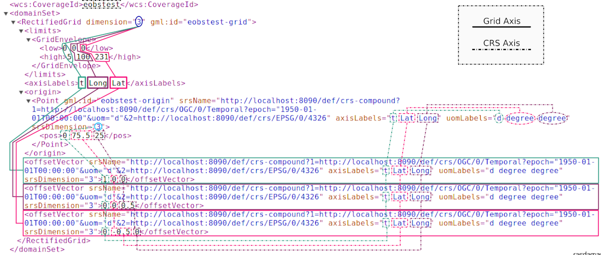
The CRS of the coverage is an (ordered) composition of a temporal CRS (linear
count of days [d] from the epoch 1950-01-01T00:00:00) and a geospatial
CRS where latitude is defined first (the well-known EPSG:4326). This means that
every tuple of spatio-temporal coordinates in the coverage’s domain will be a
3D tuple listing the count of days from 1^st^ of January 1950, then latitude
degrees then longitude degrees, like shown in the gml:origin/gml:pos
element: the origin of the 3D grid is set on 1^st^ of January 1950, 75.5
degrees north and 25 degrees east (with respect to the origin of the
cartesian CS defined in EPSG:4326).
Grid coordinates follow instead the internal grid space, which is not aware of
any spatio-temporal attribute, and follows the order of axis as they are stored
in rasdaman: in the example, it is expressed that the collection is composed
of a 6x101x232 marray, having t (time) as first axis, then Long then
Lat. The spatio-temporal coordinates are instead expressed following the
order of the CRS definition, hence with latitude degrees before longitudes.
A final remark goes to the customization of CRS (and consequently grid) axes labels, which can be particularly needed for temporal CRSs, especially in case of multiple time axis in the same CRS. Concrete CRS definitions are a static XML tree of GML elements defining axis, geographic coordinate systems, datums, and so on. The candidate standard OGC CRS Name-Type Specification offers a new kind of CRS, a parametrized CRS, which can be bound to a concrete definition, a CRS template, and which offers customization of one or more GML elements directly via key-value pairs in the query component of HTTP URL identifying the CRS.
As a practical example, we propose the complete XML definition of the parametrized CRS defining ANSI dates, identified by the URI http://rasdaman.org:8080/def/crs/OGC/0/AnsiDate:
<ParameterizedCRS xmlns:gml="http://www.opengis.net/gml/3.2"
  xmlns:xlink="http://www.w3.org/1999/xlink"
  xmlns="http://www.opengis.net/CRS-NTS/1.0"
  xmlns:epsg="urn:x-ogp:spec:schema-xsd:EPSG:1.0:dataset"
  xmlns:rim="urn:oasis:names:tc:ebxml-regrep:xsd:rim:3.0"
  gml:id="param-ansi-date-crs">
  <description>Parametrized temporal CRS of days elapsed
    from 1-Jan-1601 (00h00 UTC).</description>
  <gml:identifier codeSpace="http://www.ietf.org/rfc/rfc3986">
      http://rasdaman.org:8080/def/crs/OGC/0/AnsiDate</gml:identifier>
    <parameters>
    <parameter name="axis-label">
      <value>"ansi"</value>
      <target>//gml:CoordinateSystemAxis/gml:axisAbbrev</target>
    </parameter>
    </parameters>
    <targetCRS
      xlink:href="http://rasdaman.org:8080/def/crs/OGC/0/.AnsiDate-template"/>
</ParameterizedCRS>
This single-parameter definition allow the customization of the concrete CRS
template OGC:.AnsiDate-template (identified by
http://rasdaman.org:8080/def/crs/OGC/0/.AnsiDate-template) on its unique axis
label (crsnts:parameter/crsnts:target), via a parameter labeled
axis-label, and default value ansi.
This way, when we assign this parameterized CRS to a coverage, we can either
leave the default ansi label to the time axis, or change it to some other
value by setting the parameter in the URL query:
- default
ansiaxis label:http://rasdaman.org:8080/def/crs/OGC/0/AnsiDate - custom
ansi_dateaxis label:http://rasdaman.org:8080/def/crs/OGC/0/AnsiDate?axis-label="ansi_date"
Subsets in Petascope
We will describe how subsets (trims and slices) are treated by Petascope. Before this you will have to understand how the topology of a grid coverage is interpreted with regards to its origin, its bounding-box and the assumptions on the sample spaces of the points. Some practical examples will be proposed.
Geometric interpretation of a coverage
This section will focus on how the topology of a grid coverage is stored and how Petascope interprets it. When it comes to the so-called domainSet of a coverage (hereby also called domain, topology or geometry), Petascope follows pretty much the GML model for rectified grids: the grid origin and one offset vector per grid axis are enough to deduce the full domainSet of such (regular) grids. When it comes to referenceable grids, the domainSet still is kept in a compact vectorial form by adding weighting coefficients to one or more offset vectors.
As by `GML standard <http://www.opengeospatial.org/standards/gml>`_ a grid is a “network composed of two or more sets of curves in which the members of each set intersect the members of the other sets in an algorithmic way”. The intersections of the curves are represented by points: a point is 0D and is defined by a single coordinate tuple.
A first question arises on where to put the grid origin. The GML and GMLCOV standards say that the mapping from the domain to the range (feature space, payload, values) of a coverage is specified through a function, formally a gml:coverageFunction. From the GML standard: “If the gml:coverageFunction property is omitted for a gridded coverage (including rectified gridded coverages) the gml:startPoint is considered to be the value of the gml:low property in the gml:Grid geometry, and the gml:sequenceRule is assumed to be linear and the gml:axisOrder property is assumed to be +1 +2”.
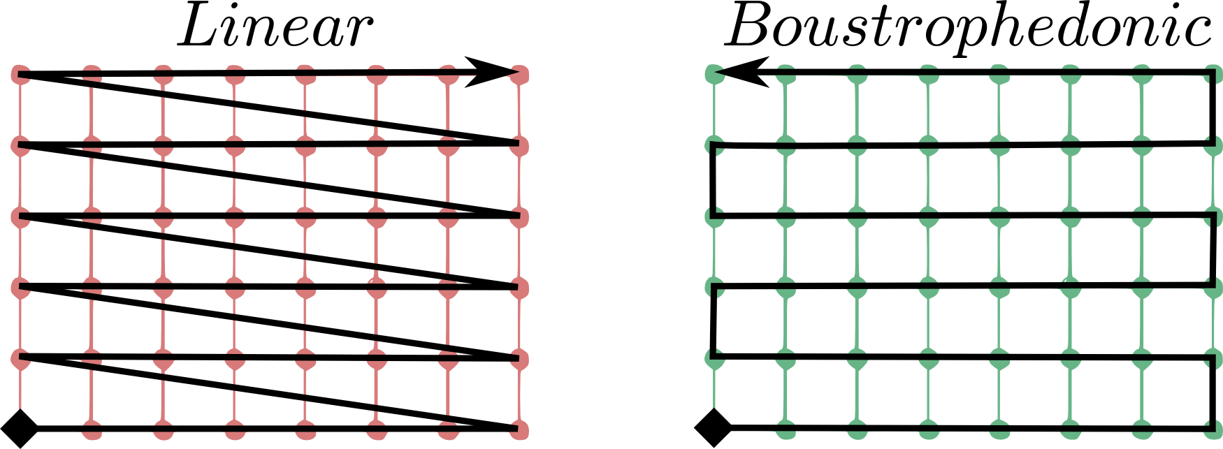
In the image, it is assumed that the first grid axis (+1) is the horizontal axis, while the second (+2) is the vertical axis; the grid starting point is the full diamond. Rasdaman uses its own grid function when listing cell values, linearly spanning the outer dimensions first, then proceeding to the innermost ones. To make it clearer, this means column-major order.
In order to have a coeherent GML output, a mapping coverage function is then declared. This can look like this in a 3D hypothetical response:
<gml:coverageFunction>
  <gml:GridFunction>
    <gml:sequenceRule axisOrder="+3 +2 +1">Linear</gml:sequenceRule>
    <gml:startPoint>0 0 0</gml:startPoint>
  </gml:GridFunction>
</gml:coverageFunction>
Coming back to the origin question on where to put the origin of our grid coverages, we have to make it coincide to what the starting value represents in rasdaman, the marray origin. As often done in GIS applications, the origin of an image is set to be its upper-left corner: this finally means that the origin of our rectified and referenceable grid coverages shall be there too in order to provide a coherent GML/GMLCOV coverage. Note that placing the origin in the upper-left corner of an image means that the offset vector along the northing axis will point South, hence will have negative norm (in case the direction of the CRS axis points North!).
When it comes to further dimensions (a third elevation axis, time, etc.),
the position of the origin depends on the way data has been ingested.
Taking the example of a time series, if the marray origin
(which we can denote as [0:0:__:0], though it is more
precisely described as [dom.lo[0]:dom.lo[1]:__:dom.lo[n])
is the earliest moment in time, then the grid origin will be
the earliest moment in the series too, and the offset vector in time
will point to the future (positive norm); in the other case, the origin
will be the latest time in the series, and its vector
will point to the past (negative norm).
To summarize, in any case the grid origin must point to the marray origin. This is important in order to properly implement our linear sequence rule.
A second question arises on how to treat coverage points: are they points or are they areas? The formal ISO term for the area of a point is sample space. We will refer to it as well as footprint or area. The GML standard provides guidance on the way to interpret a coverage: “When a grid point is used to represent a sample space (e.g. image pixel), the grid point represents the center of the sample space (see ISO 19123:2005, 8.2.2)”.
In spite of this, there is no formal way to describe GML-wise the footprint of the points of a grid. Our current policy applies distinct choices separately for each grid axis, in the following way:
- regular axis: when a grid axis has equal spacing between each of its points, then it is assumed that the sample space of the points is equal to this spacing (resolution) and that the grid points are in the middle of this interval.
- irregular axis: when a grid axis has an uneven spacing between its points, then there is no (currently implemented) way to either express or deduce its sample space, hence 0D points are assumed here (no footprint).
It is important to note that sample spaces are meaningful when areas are legal in the Coordinate Reference System (CRS): this is not the case for Index CRSs, where the allowed values are integrals only. Even on regular axes, points in an Index CRSs can only be points, and hence will have 0D footprint. Such policy is translated in practice to a point-is-pixel-center interpretation of regular rectified images.
The following art explains it visually:
KEY
          # = grid origin             o = pixel corners
          + = grid points             @ = upper-left corner of BBOX
  {v_0,v_1} = offset vectors

  |======== GRID COVERAGE MODEL =========|    |===== GRID COVERAGE + FOOTPRINTS =====|

                                             {UL}
           v_0                                 @-------o-------o-------o-------o--- -
       -------->                               |       |       |       |       |
     . #-------+-------+-------+--- -          |   #   |   +   |   +   |   +   |
 v_1 | |       |       |       |               |       |       |       |       |
     | |       |       |       .               o-------o-------o-------o-------o-- -
     V |       |       |       .               |       |       |       |       .
       +-------+-------+--- -                  |   +   |   +   |   +   |       .
       |       |       |                       |       |       |       |
       |       |       .                       o-------o-------o-------o-- -
       |       |       .                       |       |       |       .
       +-------+--- -                          |   +   |   +   .       .
       |       |                               |       |       .
       |       .                               o-------o--- -
       |       .                               |       .
       +--- -                                  .   +   .
       .                                       .
       .

  |======================================|    |======================================|
The left-side grid is the GML coverage model for a regular grid: it is a network of (rectilinear) curves, whose intersections determine the grid points ‘+’. The description of this model is what petascopedb knows about the grid.
The right-hand grid is instead how Petascope inteprets the information in petascopedb, and hence is the coverage that is seen by the enduser. You can see that, being this a regular grid, sample spaces (pixels) are added in the perception of the coverage, causing an extension of the bbox (gml:boundedBy) of half-pixel on all sides. The width of the pixel is assumed to be equal to the (regular) spacing of the grid points, hence each pixel is of size |v_0| x |v_1|, being * the norm operator.
As a final example, imagine that we take this regular 2D pattern and we build a stack of such images on irregular levels of altitude:
KEY
        # = grid origin             X = ticks of the CRS height axis
        + = grid points             O = origin of the CRS height axis
{v_0,v_2} = offset vectors


    O-------X--------X----------------------------X----------X-----X-----------> height
    |
    |       ---> v_2
    |     . #________+____________________________+__________+_____+
    | v_0 | |        |                            |          |     |
    |     V +________+____________________________+__________+_____+
    |       |        |                            |          |     |
    |       +________+____________________________+__________+_____+
    |       |        |                            |          |     |
    |       +________+____________________________+__________+_____+
    |       |        |                            |          |     |
    V       .        .                            .          .     .
 easting
In petascopedb we will need to add an other axis to the coverage topology, assigning a vector ‘v_2’ to it (we support gmlrgrid:ReferenceableGridByVectors only, hence each axis of any kind of grid will have a vector). Weighting coefficients will then determine the height of each new z-level of the cube: such heights are encoded as distance from the grid origin ‘#’ normalized by the offset vector v_2. Please note that the vector of northings v_1 is not visible due to the 2D perspective: the image is showing the XZ plane.
Regarding the sample spaces, while petascope will still assume the points are pixels on the XY plane (eastings/northings), it will instead assume 0D footprint along Z, that is along height: this means that the extent of the cube along height will exactly fit to the lowest and highest layers, and that input Z slices will have to select the exact value of an existing layer.
The latter would not hold on regular axes: this is because input subsets are targeting the sample spaces, and not just the grid points, but this is covered more deeply in the following section.
Input and output subsettings
This section will cover two different facets of the interpretation and usage of subsets: how they are formalized by Petascope and how they are adjusted. Trimming subsets ‘lo,hi’ are mainly covered here: slices do not pose many interpretative discussions.
A first point is whether an interval (a trim operation) should be (half) open or closed. Formally speaking, this determines whether the extremes of the subset should or shouldn’t be considered part of it: (lo,hi) is an open interval, [lo.hi) is a (right) open interval, and [lo,hi] is a closed interval. Requirement 38 of the WCS Core standard (OGC 09-110r4) specifies that a /subset/ is a closed interval.
A subsequent question is whether to apply the subsets on the coverage points or on their footprints. While the WCS standard does not provide recommendations, we decided to target the sample spaces, being it a much more intuitive behavior for users who might ignore the internal representation of an image and do not want to lose that “half-pixel” that would inevitably get lost if footprints were to be ignored.
We also consider here “right-open sample spaces”, so the borders of the footprints are not all part of the footprint itself: this means that two adjacent footprints will not share the border, which will instead belong to the greater point (so typically on the right side in the CRS space). A slice exactly on that border will then pick the right-hand “greater” point only. Border-points instead always include the external borders of the footprint: slices right on the native BBOX of the whole coverage will pick the border points and will not return an exception.
Clarified this, the last point is how coverage bounds are set before shipping, with respect to the input subsets. That means whether our service should return the request bounding box or the minimal bounding box.
Following the (strong) encouragement in the WCS standard itself (requirement 38 WCS Core), Petascope will fit the input subsets to the extents of sample spaces (e.g. to the pixel areas), thus returning the minimal bounding box. This means that the input bbox will usually be extended to the next footprint border. This is also a consequence of our decision to apply subsets on footprints: a value which lies inside a pixel will always select the associated grid point, even if the position of the grid point is actually outside of the subset interval.
Examples
In this section we will examine the intepretation of subsets by petascope by taking different subsets on a single dimension of 2D coverage. To appreciate the effect of sample spaces, we will first assume regular spacing on the axis, and then irregular 0D-footprints.
Test coverage information:

--------------------
mean_summer_airtemp (EPSG:4326)
Size is 886, 711
Pixel Size = (0.050000000000000,-0.050000000000000)
Upper Left  ( 111.9750000,  -8.9750000)
Lower Left  ( 111.9750000, -44.5250000)
Upper Right ( 156.2750000,  -8.9750000)
Lower Right ( 156.2750000, -44.5250000)
From this geo-information we deduce that the grid origin,
which has to be set in the upper-left corner of the image,
in the centre of the pixel are, will be:

origin(mean_summer_airtemp) = [ (111.975 + 0.025) ,  (-8.975 - 0.025) ]
                            = [  112.000          ,   -9.000          ]
Regular axis: *point-is-area*

 KEY
        o = grid point
        | = footprint border

    [=s=] = subset
        [ = subset.lo
        ] = subset.hi

 _______________________________________________________________________

          112.000   112.050   112.100   112.150   112.200
 Long:  |----o----|----o----|----o----|----o----|----o----|-- -- -
           cell0     cell1     cell2     cell3     cell4
             [s1]
                  [== s2 ===]
                  [== s3 ==]
              [==== s4 ====]
    [== s5 ==]
 _______________________________________________________________________

   s1: [112.000, 112.020]
   s2: [112.025, 112.075]
   s3: [112.025, 112.070]
   s4: [112.010, 112.070]
   s5: [111.950, 112.000]

 Applying these subsets to mean_summer_airtemp will produce the following responses:

     | GRID POINTS INCLUDED |  OUTPUT BOUNDING-BOX(Long)
 -----+----------------------+----------------------------
  s1 | cell0                |    [ 111.975, 112.025 ]
  s2 | cell1, cell2         |    [ 112.025, 112.125 ]
  s3 | cell1                |    [ 112.025, 112.075 ]
  s4 | cell0, cell1         |    [ 111.975, 112.075 ]
  s5 | cell0                |    [ 111.9
Irregular axis: *point-is-point*

      KEY
        o = grid point

    [=s=] = subset
        [ = subset.lo
        ] = subset.hi

 _______________________________________________________________________

          112.000       112.075  112.110           112.230
 Long:       o-------------o--------o-----------------o--- -- -
           cell0         cell1    cell2             cell3
             [s1]
               [== s2 ===]
                    [== s3 ==]
          [======= s4 =======]
    [== s5 ==]
 _______________________________________________________________________

   s1: [112.000, 112.020]
   s2: [112.010, 112.065]
   s3: [112.040, 112.090]
   s4: [111.970, 112.090]
   s5: [111.920, 112.000]

Applying these subsets to mean_summer_airtemp will produce the following responses (please note tickets #681 and #682):

     | GRID POINTS INCLUDED |  OUTPUT BOUNDING-BOX(Long)
 -----+----------------------+----------------------------
  s1 | cell0                |    [ 112.000, 112.000 ]
  s2 | --- (WCSException)   |    [ --- ]
  s3 | cell1                |    [ 112.075, 112.075 ]
  s4 | cell0, cell1         |    [ 112.000, 112.075 ]
  s5 | cell0                |    [ 112.000, 112.000 ]
CRS management
Petascope relies on a [SecoreUserGuide SECORE] Coordinate Reference System (CRS)
resolver that can provide proper metadata on, indeed, coverage’s native CRSs.
One could either [SecoreDevGuide deploy] a local SECORE instance, or use the
official OGC SECORE resolver
(http://www.opengis.net/def/crs/). CRS resources are identified then by HTTP
URIs, following the related OGC policy document of 2011, based on the White
Paper ‘OGC Identifiers - the case for http URIs’. These HTTP URIs
must resolve to GML resources that describe the CRS, such as
http://rasdaman.org:8080/def/crs/EPSG/0/27700 that themselves contain only
resolvable HTTP URIs pointing to additional definitions within the CRS; so for
example http://www.epsg-registry.org/export.htm?gml=urn:ogc:def:crs:EPSG::27700
is not allowed because, though it is a resolvable HTTP URI pointing at a GML
resource that describes the CRS, internally it uses URNs which SECORE is unable
to resolve.
OGC Web Services
WCS
“The OpenGIS Web Coverage Service Interface Standard (WCS) defines a standard interface and operations that enables interoperable access to geospatial coverages.” (WCS standards)
Metadata regarding the range (feature space) of a coverage "myCoverage" is a
fundamental part of a GMLCOV coverage model.
Responses to WCS DescribeCoverage and GetCoverage will show such information
in the gmlcov:rangeType element, encoded as fields of the OGC SWE data
model.
For instance, the range type of a test coverage mr, associated with the
primitive quantity with unsigned char values is the following:
<gmlcov:rangeType>
    <swe:DataRecord>
    <swe:field name="value">
        <swe:Quantity definition="http://www.opengis.net/def/dataType/OGC/0/unsignedByte">
        <swe:label>unsigned char</swe:label>
        <swe:description>primitive</swe:description>
        <swe:uom code="10^0"/>
        <swe:constraint>
          <swe:AllowedValues>
            <swe:interval>0 255</swe:interval>
          </swe:AllowedValues>
        </swe:constraint>
        </swe:Quantity>
    </swe:field>
    </swe:DataRecord>
</gmlcov:rangeType>
Note that a quantity can be associated with multiple allowed intervals, as by SWE specifications.
Declarations of NIL values are also possible: one or more values representing not available data or which have special meanings can be declared along with related reasons, which are expressed via URIs (see http://www.opengis.net/def/nil/OGC/0/ for official NIL resources provided by OGC).
You can use http://yourserver/rasdaman/ows as service endpoints to which to
send WCS requests, e.g.
http://yourserver/rasdaman/ows?service=WCS&version=2.0.1&request=GetCapabilities
See example queries in the WCS systemtest which send KVP (key value pairs) GET request and XML POST request to Petascope.
WCPS
“The OpenGIS Web Coverage Service Interface Standard (WCS) defines a protocol-independent language for the extraction, processing, and analysis of multi-dimensional gridded coverages representing sensor, image, or statistics data. Services implementing this language provide access to original or derived sets of geospatial coverage information, in forms that are useful for client-side rendering, input into scientific models, and other client applications. Further information about WPCS can be found at the WCPS Service page of the OGC Network. (http://www.opengeospatial.org/standards/wcps)
The WCPS language is independent from any particular request and response encoding, allowing embedding of WCPS into different target service frameworks like WCS and WPS. The following documents are relevant for WCPS; they can be downloaded from www.opengeospatial.org/standards/wcps:
- OGC 08-068r2: The protocol-independent (“abstract”) syntax definition; this is the core document. Document type: IS (Interface Standard.
- OGC 08-059r3: This document defines the embedding of WCPS into WCS by specifying a concrete protocol which adds an optional ProcessCoverages request type to WCS. Document type: IS (Interface Standard).
- OGC 09-045: This draft document defines the embedding of WCPS into WPS as an application profile by specifying a concrete subtype of the Execute request type.
There are a online demo and online tutorial; see also the WCPS manual and tutorial.
The petascope implementation supports both Abstract (example) and XML syntaxes (example). For guidelines on how to safely build and troubleshoot WCPS query with Petascope, see this topic in the mailing-list.
The standard for WCPS GET request is
http://yourserver/rasdaman/ows?service=WCS&version=2.0.1
  &request=ProcessCoverage&query=YOUR\_WCPS\_QUERY
You can use http://your.server/rasdaman/ows/wcps as a shortcut
service endpoint to which to send WCPS requests. This is not an OGC
standard for WCPS but is kept for testing purpose for WCPS queries.
The following form is equivalent to the previous one:
http://yourserver/rasdaman/ows/wcps?query=YOUR\_WCPS\_QUERY
WMS
“The OpenGIS Web Map Service Interface Standard (WMS) provides a simple HTTP interface for requesting geo-registered map images from one or more distributed geospatial databases. A WMS request defines the geographic layer(s) and area of interest to be processed. The response to the request is one or more geo-registered map images (returned as JPEG, PNG, etc) that can be displayed in a browser application. The interface also supports the ability to specify whether the returned images should be transparent so that layers from multiple servers can be combined or not.”
Petascope supports WMS 1.3.0. Some resources:
Administration
The WMS 1.3 is self-administered by all intents and purposes, the
database schema is created automatically and updates each time the
Petascope servlet starts if necessary. The only input needed from the
administrator is the service information which should be filled in
$RMANHOME/etc/wms_service.properties before the servlet is started.
Data ingestion & removal
Layers can be easily created from existing coverages in WCS. This has several advantages:
- Creating the layer is extremely simple and can be done by both humans and machines.
- The possibilities of inserting data into WCS are quite advanced (see wiki:WCSTImportGuide).
- Data is not duplicated among the services offered by Petascope.
Possible WMS requests:
- The
InsertWCSLayerrequest will create a new layer from an existing coverage without an associated WMS layer served by the web coverage service offered by petascope. Example:
http://example.org/rasdaman/ows?service=WMS&version=1.3.0
       &request=InsertWCSLayer&wcsCoverageId=MyCoverage
- To update an existing WMS layer from an existing coverage with
an associated WMS layer use
UpdateWCSLayerrequest. Example:
http://example.org/rasdaman/ows?service=WMS&version=1.3.0
        &request=UpdateWCSLayer&wcsCoverageId=MyCoverage
- To remove a layer, just delete associated coverage. Example:
http://example.org/rasdaman/ows?service=WCS&version=2.0.1
        &request=DeleteCoverage&coverageId=MyCoverage
Transparent nodata value
By adding a parameter transparent=true to WMS requests, the returned image
will have NoData Value=0 in the bands’ metadata, so the WMS client will
consider all the pixels with 0 value as transparent. E.g:
http://localhost:8080/rasdaman/ows?service=WMS&version=1.3.0
    &request=GetMap&layers=waxlake1
    &bbox=618887,3228196,690885,%203300195.0
    &crs=EPSG:32615&width=600&height=600&format=image/png
    &TRANSPARENT=TRUE
Style creation
Styles can be created for layers using rasql and WCPS query fragments. This allows users to define several visualization options for the same dataset in a flexible way. Examples of such options would be color classification, NDVI detection etc. The following HTTP request will create a style with the name, abstract and layer provided in the KVP parameters below
Note
For Tomcat version 7+ it requires the query (WCPS/rasql fragment) to be encoded correctly. Please use this website http://meyerweb.com/eric/tools/dencoder/ to encode your query first:
WCPS query fragment example (since rasdaman 9.5):
 http://localhot:8080/rasdaman/ows?
     service=WMS&
     version=1.3.0&
     request=InsertStyle&
     name=wcpsQueryFragment&
     layer=test_wms_4326&
     abstract=This style marks the areas where fires are in progress with the color red&
     wcpsQueryFragment=switch case $c > 1000 return {red: 107; green:17; blue:68}
     default return {red: 150; green:103; blue:14})

The variable $c will be replaced by a layer name when sending a GetMap request
containing this layer's style.
Rasql query fragment examples:
http://example.org/rasdaman/ows?service=WMS&version=1.3.0&request=InsertStyle
    &name=FireMarkup
    &layer=dessert_area
    &abstract=This style marks the areas where fires are in progress with the color red
    &rasqlTransformFragment=case $Iterator when ($Iterator + 2) > 200 then {255, 0, 0}
    else {0, 255, 0} end
The variable
$Iteratorwill be replaced with the actual name of the rasdaman collection and the whole fragment will be integrated inside the regularGetMaprequest.
Removal
To remove a particular style you can use a DeleteStyle request. Note
that this is a non-standard extension of WMS 1.3.
http://example.org/rasdaman/ows?service=WMS&version=1.3.0
    &request=DeleteStyle&layer=dessert_area&style=FireMarkup
3D+ coverage as WMS layer
Petascope allows to import a 3D+ coverage as a WMS layer. The user can specify
"wms_import": true in the ingredients file when importing data with
wcst_import.sh for 3D+ coverage with regular_time_series,
irregular_time_series and general_coverage recipes.
For example
you find an irregular_time_series 3D coverage from 2D geotiff files use case.
Once the data coverage is ingested, the user can send GetMap requests
on non-geo-referenced axes according to the OGC WMS 1.3.0 standard.
The table below shows the subset parameters for different axis types:
| Axis Type | Subset parameter | |
|---|---|---|
| Time | time=… | |
| Elevation | elevation=… | |
| Other | dim_AxisName=… (e.g dim_pressure=…) | |
According to the WMS 1.3.0 specification, the subset for non-geo-referenced axes can have these formats:
- Specific value (value1): time=‘2012-01-01T00:01:20Z, dim_pressure=20,…
- Range values (min/max): time=‘2012-01-01T00:01:20Z’/‘2013-01-01T00:01:20Z, dim_pressure=20/30,…
- Multiple values (value1,value2,value3,…): time=‘2012-01-01T00:01:20Z, ‘2013-01-01T00:01:20Z, dim_pressure=20,30,60,100,…
- Multiple range values (min1/max1,min2/max2,…): dim_pressure=20/30,40/60,…
Note
A GetMap request is always 2D, so if a non-geo-referenced axis
is omitted from the request it will be considered as a slice
on the upper bound of this axis (e.g. in a time-series it will
return the slice for the latest date).
GetMap request examples:
- Multiple values on time axis of 3D coverage.
* Multiple values on time, dim_pressure axes of 4d coverage.
Testing the WMS
You can test the service using your favorite WMS client or directly through a GetMap request like the following:
http://example.org/rasdaman/ows?service=WMS&version=1.3.0&request=GetMap
    &layers=MyLayer
    &bbox=618885.0,3228195.0,690885.0,3300195.0
    &crs=EPSG:32615
    &width=600
    &height=600
    &format=image/png
Errors and Workarounds
- Cannot load new WMS layer in QGIS
- In this case, the problem is due to QGIS caching the WMS GetCapabilities from the last request so the new layer does not exist (see here for clear caching solution: http://osgeo-org.1560.x6.nabble.com/WMS-provider-Cannot-calculate-extent-td5250516.html)
WCS-T
The WCS Transaction extension (WCS-T) defines a standard way of inserting, deleting and updating coverages via a set of web requests. This guide describes the request types that WCS-T introduces and shows the steps necessary to import coverage data into a rasdaman server, data which is then available in the server’s WCS offerings.
Supported coverage data format
Currently, WCS-T supports coverages in GML format for importing. The metadata of the coverage is thus explicitly specified, while the raw cell values can be stored either explicitly in the GML body, or in an external file linked in the GML body, as shown in the examples below. The format of the file storing the cell values must be one supported by the GDAL library (http://www.gdal.org/formats_list.html), such as TIFF / GeoTIFF, JPEG, JPEG2000, PNG etc.
Inserting coverages
Inserting a new coverage into the server’s WCS offerings is done using
the InsertCoverage request.
Standard parameters:
| Request Parameter | Value | Description | Required |
|---|---|---|---|
| service | WCS | Yes | |
| version | 2.0.1 or later | Yes | |
| request | InsertCoverage | Yes | |
| inputCoverageRef | a valid url. | Url pointing to the GML coverage to be inserted. | One of inputCoverageRef or inputCoverage is required |
| inputCoverage | a coverage in GML format | The coverage to be inserted, in GML format. | One of inputCoverageRef or inputCoverage is required |
| useId | new or existing | Indicates wheter to use the coverage id from the coverage body, or tells the server to generate a new one. | No |
Vendor specific parameters:
| Request Parameter | Value | Description | Required |
|---|---|---|---|
| pixelDataType | any GDAL supported data type | In cases where cell values are given in the GML body, the datatype can be indicated through this parameter. If omitted, it defaults to Byte. | No |
| tiling | same as rasdaman tiling clause wiki:Tiling | Indicates the tiling of the array holding the cell values. | No |
The response of a successful coverage request is the coverage id of the newly inserted coverage.
Examples
The following example shows how to insert the coverage available at: http://schemas.opengis.net/gmlcov/1.0/examples/exampleRectifiedGridCoverage-1.xml. The tuple list is given in the GML body.
http://localhost:8080/rasdaman/ows?service=WCS&version=2.0.1&request=InsertCoverage
    &coverageRef=http://schemas.opengis.net/gmlcov/1.0/examples/exampleRectifiedGridCoverage-1.xml
The following example shows how to insert a coverage stored on the server on which rasdaman runs. The cell values are stored in a TIFF file (attachment:myCov.gml), the coverage id is generated by the server and aligned tiling is used for the array storing the cell values.
http://localhost:8080/rasdaman/ows?service=WCS&version=2.0.1&request=InsertCoverage
    &coverageRef=file:///etc/data/myCov.gml&useId=new&tiling=aligned [0:500, 0:500]
Coming soon: the same operation, but via a POST XML request to http://localhost:8080/rasdaman/ows:
<?xml version="1.0" encoding="UTF-8"?>
    <wcs:InsertCoverage
    xmlns:xsi="http://www.w3.org/2001/XMLSchema-instance"
    xmlns:wcs="http://www.opengis.net/wcs/2.0"
    xmlns:gml="http://www.opengis.net/gml/3.2"
    xsi:schemaLocation="http://schemas.opengis.net/wcs/2.0 ../wcsAll.xsd"
    service="WCS" version="2.0.1">
  <wcs:coverage>here goes the contents of myCov.gml</wcs:coverage>
  <wcs:useId>
    new
  </wcs:useId>
</wcs:InsertCoverage>
Deleting coverages
To delete a coverage (along with the corresponding rasdaman collection), use the
standard DeleteCoverage WCS-T request. For example, the coverage
‘test_mr’ can be deleted with a request as following:
http://yourserver/rasdaman/ows?service=WCS&version=2.0.1
  &request=DeleteCoverage&coverageId=test_mr
Deleting coverages is also possible from the WS-client frontend available at
http://yourserver/rasdaman/ows (WCS > DeleteCoverage tab).
Non-standard requests
WMS
The following requests are used to create/delete downscaled coverages which are used for WMS pyramids feature.
InsertScaleLevel: create a downscaled collection for a specific coverage and given level; e.g. to create a downscaled coverage of test_world_map_scale_levels that is 4x smaller:
http://localhost:8082/rasdaman/ows?service=WCS&version=2.0.1
&request=InsertScaleLevel
&coverageId=test_world_map_scale_levels
&level=4
DeleteScaleLevel: delete an existing downscaled coverage at a given level; e.g. to delete downscaled level 4 of coverage test_world_map_scale_levels:
http://localhost:8082/rasdaman/ows?service=WCS&version=2.0.1
&request=DeleteScaleLevel
&coverageId=test_world_map_scale_levels
&level=4`
Non-standard functionality
Clipping in petascope
WCS and WCPS services in Petascope support the WKT format for clipping with
MultiPolygon (2D), Polygon (2D) and LineString (1D+). The result of
MultiPolygon and Polygon is always a 2D coverage, and LineString results in a
1D coverage.
Petascope also supports curtain and corridor clippings by Polygon
and Linestring on 3D+ coverages by Polygon (2D) and Linestring (1D).
The result of curtain clipping has same dimensionality as the input coverage
and the result of corridor clipping is always a 3D coverage
with the first axis being the trackline of the corridor by convention.
Below you find the documentation for WCS and WCPS with a few simple examples; an interactive demo is available here.
WCS
Clipping can be done by adding a &clip= parameter to the request. If the
subsettingCRS parameter is specified then this CRS applies to the clipping
WKT as well, otherwise it is assumed that the WKT is in the native coverage CRS.
Examples
Polygon clipping on coverage with nativeCRS
EPSG:4326.http://localhost:8080/rasdaman/ows& service=WCS& version=2.0.1& request=GetCoverage& coverageId=test_wms_4326& clip=POLYGON((55.8 -96.6, 15.0 -17.3))& format=image/png
Polygon clipping with coordinates in
EPSG:3857(fromsubsettingCRSparameter) on coverage with nativeCRSEPSG:4326.http://localhost:8080/rasdaman/ows& service=WCS& version=2.0.1& request=GetCoverage& coverageId=test_wms_4326& clip=POLYGON((13589894.568 -2015496.69612, 15086830.0246 -1780682.3822))& subsettingCrs=http://opengis.net/def/crs/EPSG/0/3857& format=image/png
Linestring clipping on a 3D coverage
(axes: X, Y, ansidate).http://localhost:8080/rasdaman/ows& service=WCS& version=2.0.1& request=GetCoverage& coverageId=test_irr_cube_2& clip=LineStringZ(75042.7273594 5094865.55794 "2008-01-01T02:01:20.000Z", 705042.727359 5454865.55794 "2008-01-08T00:02:58.000Z")& format=text/csv
Multipolygon clipping on 2D coverage
http://localhost:8080/rasdaman/ows&
service=WCS&
version=2.0.1&
request=GetCoverage&
coverageId=test_mean_summer_airtemp&
clip=Multipolygon( ((-23.189600 118.432617, -27.458321 117.421875,
                     -30.020354 126.562500, -24.295789 125.244141)),
                   ((-27.380304 137.768555, -30.967012 147.700195,
                     -25.491629 151.259766, -18.050561 142.075195)) )&
format=image/png
Curtain clipping by a Linestring on 3D coverage
http://localhost:8080/rasdaman/ows&
service=WCS&
version=2.0.1&
request=GetCoverage&
coverageId=test_eobstest&
clip=CURTAIN( projection(Lat, Long), linestring(25 41, 30 41, 30 45, 30 42) )&
format=text/csv
Curtain clipping by a Polygon on 3D coverage
http://localhost:8080/rasdaman/ows&
service=WCS&
version=2.0.1&
request=GetCoverage&
coverageId=test_eobstest&
clip=CURTAIN(projection(Lat, Long), Polygon((25 40, 30 40, 30 45, 30 42)))&
format=text/csv
Corridor clipping by a Linestring on 3D coverage
http://localhost:8080/rasdaman/ows&
service=WCS&
version=2.0.1&
request=GetCoverage&
coverageId=test_irr_cube_2&
clip=corridor( projection(E, N),
     LineString(75042.7273594  5094865.55794 "2008-01-01T02:01:20.000Z",
                75042.7273594 5194865.55794 "2008-01-01T02:01:20.000Z"),
     LineString(75042.7273594 5094865.55794, 75042.7273594 5094865.55794,
                85042.7273594 5194865.55794, 95042.7273594 5194865.55794)
    )&
format=application/gml+xml
Corridor clipping by a Polygon on 3D coverage
http://localhost:8080/rasdaman/ows&
service=WCS&
version=2.0.1&
request=GetCoverage&
coverageId=test_eobstest&
clip=corridor( projection(Lat, Long),
     LineString(26 41 "1950-01-01", 28 41 "1950-01-02"),
     Polygon((25 40, 30 40, 30 45, 25 45)), discrete )&
format=application/gml+xml
WCPS
A special function that works similarly as in the case of WCS is provided with the following signature:
clip( coverageExpression, wkt [, subsettingCrs ] )
where
coverageExpressionis some coverage variable likecovor an expression that results in a coverage like `cos(cov+10)`wktis a valid WKT construct, e.g.POLYGON((...)),LineString(...)subsettingCrsis an optional parameter to specify the CRS for the coordinates inwkt(e.g “http://opengis.net/def/crs/EPSG/0/4326”).
Examples
Polygon clipping with coordinates in
EPSG:4326on coverage with nativeCRSEPSG:3857.for c in (test_wms_3857) return encode( clip(c, POLYGON(( -17.8115 122.0801, -15.7923 135.5273, -24.8466 151.5234, -19.9733 137.4609, -33.1376 151.8750, -22.0245 135.6152, -37.5097 145.3711, -24.4471 133.0664, -34.7416 135.8789, -25.7207 130.6934, -31.8029 130.6934, -26.5855 128.7598, -32.6949 125.5078, -26.3525 126.5625, -35.0300 118.2129, -25.8790 124.2773, -30.6757 115.4004, -24.2870 122.3438, -27.1374 114.0820, -23.2413 120.5859, -22.3501 114.7852, -21.4531 118.5645 )), "http://opengis.net/def/crs/EPSG/0/4326" ) , "png")Linestring clipping on 3D coverage (axes:
X, Y, datetime).for c in (test_irr_cube_2) return encode( clip(c, LineStringZ(75042.7273594 5094865.55794 "2008-01-01T02:01:20.000Z", 705042.727359 5454865.55794 "2008-01-08T00:02:58.000Z")) , "csv")Linestring clipping on 2D coverage
with coordinates(axes:X, Y).for c in (test_mean_summer_airtemp) return encode( clip(c, LineString(-29.3822 120.2783, -19.5184 144.4043)) with coordinates , "csv")
In this case the geo coordinates of the values on the linestring will be included as well in the result. The first band of the result will hold the X coordinate, second band the Y coordinate, and the remaining bands the original cell values. Example output for the above query:
"-28.975 119.975 90","-28.975 120.475 84","-28.475 120.975 80", ...
Multipolygon clipping on 2D coverage.
for c in (test_mean_summer_airtemp) return encode(
 clip(c, Multipolygon(
      (( -20.4270 131.6931, -28.4204 124.1895,
         -27.9944 139.4604, -26.3919 129.0015 )),
      (( -20.4270 131.6931, -19.9527 142.4268,
         -27.9944 139.4604, -21.8819 140.5151 )) ) )
, "png")
Curtain clipping by a Linestring on 3D coverage
for c in (test_eobstest) return encode(
   clip(c, CURTAIN(projection(Lat, Long),
        linestring(25 40, 30 40, 30 45, 30 42) ) ), "csv")
Curtain clipping by a Polygon on 3D coverage
for c in (test_eobstest) return encode(
 clip(c, CURTAIN(projection(Lat, Long),
      Polygon((25 40, 30 40, 30 45, 30 42)) ) ), "csv")
Corridor clipping by a Linestring on 3D coverage
for c in (test_irr_cube_2) return encode(
 clip( c, corridor( projection(E, N),
       LineString(75042.7273594  5094865.55794 "2008-01-01T02:01:20.000Z",
                  75042.7273594 5194865.55794 "2008-01-01T02:01:20.000Z"),
       Linestring(75042.7273594 5094865.55794, 75042.7273594 5094865.55794,
                  85042.7273594 5194865.55794, 95042.7273594 5194865.55794) ) )
, "gml")
Corridor clipping by a Polygon on 3D coverage (geo CRS:
EPSG:4326) with input geo coordinates inEPSG:3857.for c in (test_eobstest) return encode( clip( c, corridor( projection(Lat, Long), LineString(4566099.12252 2999080.94347 "1950-01-01", 4566099.12252 3248973.78965 "1950-01-02"), Polygon((4452779.63173 2875744.62435, 4452779.63173 3503549.8435, 5009377.0857 3503549.8435, 5009377.0857 2875744.62435)) ), "http://localhost:8080/def/crs/EPSG/0/3857" ) , "gml")
Data import
Raster data (tiff, netCDF, grib, …) can be imported in petascope through its
WCS-T standard implementation. For convenience rasdaman provides the
wcst_import.sh tool, which hides the complexity of building WCS-T requests
for data import. Internally, WCS-T ingests the coverage geo-information into
petascopedb, while the raster data is ingested into rasdaman.
Building large timeseries/datacubes, mosaics, etc. and keeping them up-to-date as new data becomes available is supported even for complex data formats and file/directory organizations. The systemtest contains many examples for importing different types of data. Following is a detailed documentation on how to setup an ingredients file for your dataset.
Introduction
The wcst_import.sh tool introduces two concepts:
- - Recipe - A recipe is a class implementing the BaseRecipe that based on a set of
- parameters (ingredients) can import a set of files into WCS forming a well defined coverage (image, regular timeseries, irregular timeseries etc);
- - Ingredients - An ingredients file is a JSON file containing a set of parameters
- that define how the recipe should behave (e.g. the WCS endpoint, the coverage name, etc.)
To execute an ingredients file in order to import some data:
$ wcst_import.sh path/to/my_ingredients.json
Alternatively, wcst_import.sh tool can be started as a daemon as follows:
$ wcst_import.sh path/to/my_ingredients.json --daemon start
or as a daemon that is “watching” for new data at some interval (in seconds):
$ wcst_import.sh path/to/my_ingredients.json --watch <interval>
For further informations regarding wcst_import.sh commands and usage:
$ wcst_import.sh --help
The workflow behind is depicted approximately on Figure 29.
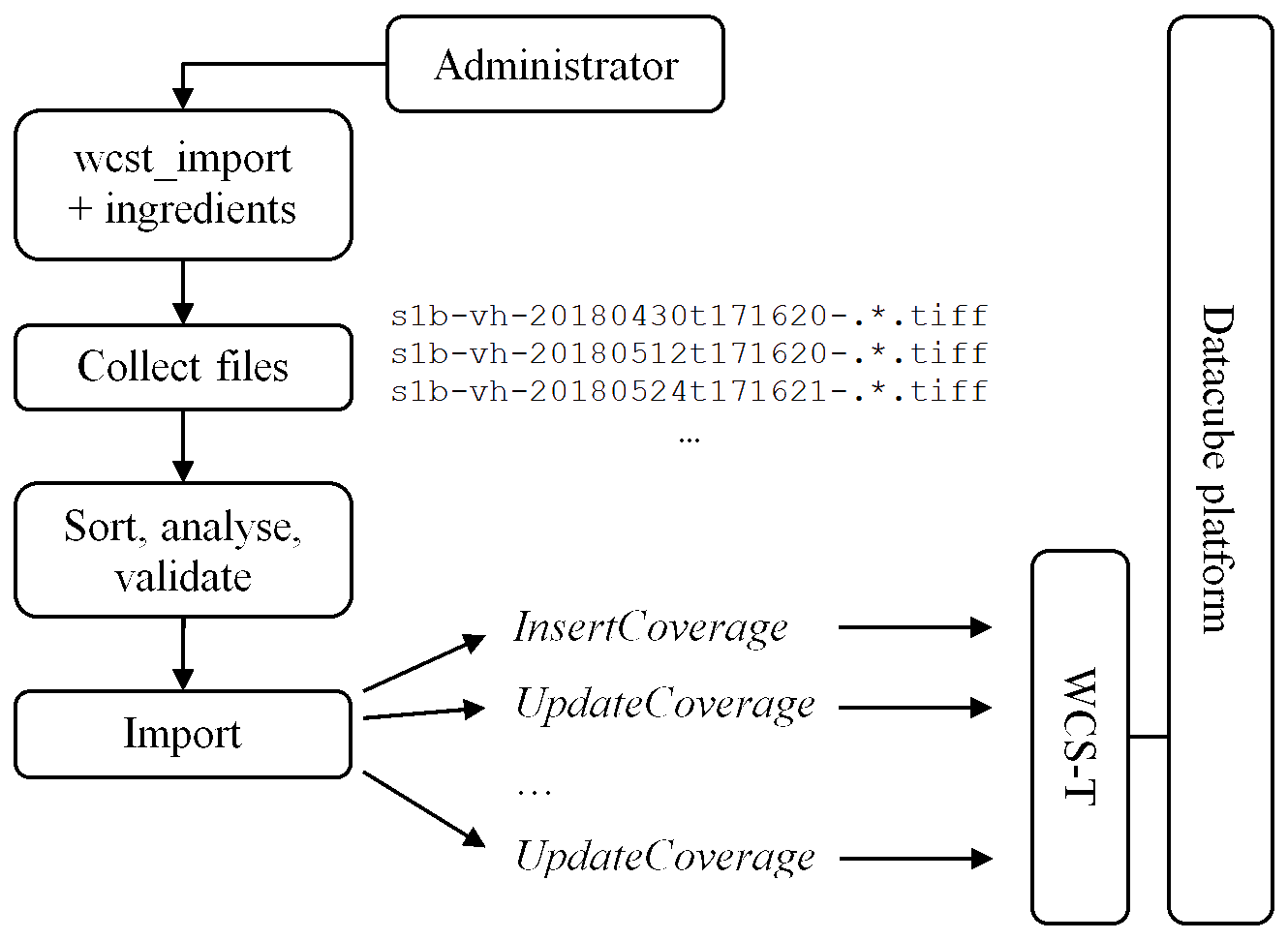
Figure 29 Ingestion process with wcst_import.sh
An ingredients file with all possible options can be found here; in the same directory you will find several examples for different recipes.
Recipes
As of now, these recipes are provided:
For each one of these there is an ingredients example under the ingredients/ directory, together with an example for the available parameters Further on each recipe type is described in turn.
Note
The comments syntax using “//comment explaining things” in the examples is not valid json so they need to be removed if you copy the parameters.
… data-import-common-options:
Common options
Some options are commonly applicable to all recipes.
“config” section
service_url- The endpoint of the WCS service with the WCS-T extension enabledmock- Print WCS-T requests but do not execute anything if set totrue. Set tofalseby default.automated- Set totrueto avoid any interaction during the ingestion process. Useful in production environments for automated deployment for example. By default it isfalse, i.e. user confirmation is needed to execute the ingestion.default_null_values- This parameter adds default null values for bands that do not have a null value provided by the file itself. The value for this parameter should be an array containing the desired null value either as a closed intervallow:highor single values. E.g. for a coverage with 3 bands"default_null_values": [ "9995:9999", "-9, -10, -87", 3.14 ],
Note, if set this parameter will override the null/nodata values present in the input files.
tmp_directory- Temporary directory in which gml and data files are created; should be readable and writable by rasdaman, petascope and current user. By default this is/tmp.crs_resolver- The crs resolver to use for generating WCS-T request. By default it is determined from thepetascope.propertiessetting.url_root- In case the files are exposed via a web-server and not locally, you can specify the root file url here; the default value is"file://".skip- Set totrueto ignore files that failed to import; by default it isfalse, i.e. the ingestion is terminated when a file fails to import.retry- Set totrueto retry a failed request. The number of retries is either 5, or the value of settingretriesif specified. This is set tofalseby default.retries- Control how many times to retry a failed WCS-T request; set to 5 by default.retry_sleep- Set number of seconds to wait before retrying after an error; a floating-point number can also be specified for sub-second precision. Default values is 1.track_files- Set totrueto allow files to be tracked in order to avoid reimporting already imported files. This setting is enabled by default.resumer_dir_path- The directory in which to store the track file. By default it will be stored next to the ingredients file.slice_restriction- Limit the slices that are imported to the ones that fit in a specified bounding box. Each subset in the bounding box should be of form{ "low": 0, "high": <max> }, where low/high are given in the axis format. Example:"slice_restriction": [ { "low": 0, "high": 36000 }, { "low": 0, "high": 18000 }, { "low": "2012-02-09", "high": "2012-12-09", "type": "date" } ]
description_max_no_slices- maximum number of slices (files) to show for preview before starting the actual ingestion.subset_correction(deprecated since rasdaman v9.6) - In some cases the resolution is small enough to affect the precision of the transformation from domain coordinates to grid coordinates. To allow for corrections that will make the import possible, set this parameter totrue.insitu- Set totrueto register files in-situ, rather than ingest them in rasdaman. Note: only applicable to rasdaman enterprise.
“recipes” / “options” section
import_order- Allow to sort the input files (ascending(default) ordescending).Currently, it sorts by datetime which allows to import coverage from the first date or the recent date. Example:"import_order": "descending"
tiling- Specifies the tile structure to be created for the coverage in rasdaman. You can set arbitrary tile sizes for the tiling option only if the tile name isALIGNED. Example:"tiling": "ALIGNED [0:0, 0:1023, 0:1023] TILE SIZE 5000000"
For more information on tiling please check the Storage Layout Language
wms_import- If set totrue, after importing data to coverage, it will also create a WMS layer from the imported coverage and populate metadata for this layer. After that, this layer will be available from WMS GetCapabilties request. Example:"wms_import": true
scale_levels- Enable the WMS pyramids feature. Syntax:"scale_levels": [ level1, level2, ... ]
Mosaic map
Well suited for importing a tiled map, not necessarily continuous; it will place all input files given under a single coverage and deal with their position in space. Parameters are explained below.
{
  "config": {
    // The endpoint of the WCS service with the WCS-T extension enabled
    "service_url": "http://localhost:8080/rasdaman/ows",
    // If set to true, it will print the WCS-T requests and will not
    // execute them. To actually execute them set it to false.
    "mock": true,
    // If set to true, the process will not require any user confirmation.
    // This is useful for production environments when deployment is automated.
    "automated": false
  },
  "input": {
    // The name of the coverage; if the coverage already exists,
    // it will be updated with the new files
    "coverage_id": "MyCoverage",
    // Absolute or relative (to the ingredients file) path or regex that
    // would work with the ls command. Multiple paths separated by commas
    // can be specified.
    "paths": [ "/var/data/*" ]
  },
  "recipe": {
    // The name of the recipe
    "name": "map_mosaic",
    "options": {
      // The tiling to be applied in rasdaman
      "tiling": "ALIGNED [0:511, 0:511]"
    }
  }
}
Regular timeseries
Well suited for importing multiple 2-D slices created at regular intervals of time (e.g sensor data, satelite imagery etc) as 3-D cube with the third axis being a temporal one. Parameters are explained below
{
  "config": {
    // The endpoint of the WCS service with the WCS-T extension enabled
    "service_url": "http://localhost:8080/rasdaman/ows",
    // If set to true, it will print the WCS-T requests and will not
    // execute them. To actually execute them set it to false.
    "mock": true,
    // If set to true, the process will not require any user confirmation.
    // This is useful for production environments when deployment is automated.
    "automated": false
  },
  "input": {
    // The name of the coverage; if the coverage already exists,
    // it will be updated with the new files
    "coverage_id": "MyCoverage",
    // Absolute or relative (to the ingredients file) path or regex that
    // would work with the ls command. Multiple paths separated by commas
    // can be specified.
    "paths": [ "/var/data/*" ]
  },
  "recipe": {
    // The name of the recipe
    "name": "time_series_regular",
    "options": {
      // Starting date for the first spatial slice
      "time_start": "2012-12-02T20:12:02",
      // Format of the time provided above: `auto` to try to guess it,
      // otherwise use any combination of YYYY:MM:DD HH:mm:ss
      "time_format": "auto",
      // Distance between each slice in time, granularity seconds to days
      "time_step": "2 days 10 minutes 3 seconds",

      // CRS to be used for the time axis
      "time_crs": "http://localhost:8080/def/crs/OGC/0/AnsiDate",
      // The tiling to be applied in rasdaman
      "tiling": "ALIGNED [0:1000, 0:1000, 0:2]"
    }
  }
}
Irregular timeseries
Well suited for importing multiple 2-D slices created at irregular intervals of time into a 3-D cube with the third axis being a temporal one. There are two types of time parameters in “options”, one needs to be choosed according to the particular use case:
tag_namewithTIFFTAG_DATETIMEinside image’s metadata (can be checked with gdalinfo filename, not every image has this parameters). Here is an example with the “tag_name” optionfilenameallows an arbitrary pattern to extract the time information from the data file paths. Here is an example with the “filename” option
{
  "config": {
    // The endpoint of the WCS service with the WCS-T extension enabled
    "service_url": "http://localhost:8080/rasdaman/ows",
    // If set to true, it will print the WCS-T requests and will not
    // execute them. To actually execute them set it to false.
    "mock": true,
    // If set to true, the process will not require any user confirmation.
    // This is useful for production environments when deployment is automated.
    "automated": false
  },
  "input": {
    // The name of the coverage; if the coverage already exists,
    // it will be updated with the new files
    "coverage_id": "MyCoverage",
    // Absolute or relative (to the ingredients file) path or regex that
    // would work with the ls command. Multiple paths separated by commas
    // can be specified.
    "paths": [ "/var/data/*" ]
  },
  "recipe": {
    // The name of the recipe
    "name": "time_series_irregular",
    "options": {
      // Information about the time parameter, two options (pick one!)

      // 1. Get the date for the slice from a tag that can be read by GDAL
      "time_parameter": {
        "metadata_tag": {
          // The name of such a tag
          "tag_name": "TIFFTAG_DATETIME"
        },
        // The format of the datetime value in the tag
        "datetime_format": "YYYY:MM:DD HH:mm:ss"
      },

      // 2. Extract the date/time from the file name
      "time_parameter" :{
        "filename": {
          // The regex has to contain groups of tokens, separated by parentheses.
          "regex": "(.*)_(.*)_(.+?)_(.*)",
          // Which regex group to use for retrieving the time value
          "group": "2"
        },
      }

      // CRS to be used for the time axis
      "time_crs": "http://localhost:8080/def/crs/OGC/0/AnsiDate",
      // The tiling to be applied in rasdaman
      "tiling": "ALIGNED [0:1000, 0:1000, 0:2]"
    }
  }
}
General coverage
The general recipe aims to be a highly flexible recipe that can handle any kind of data files (be it 2D, 3D or n-D) and model them in coverages of any dimensionality. It does that by allowing users to define their own coverage models with any number of bands and axes and fill the necesary coverage information through the so called ingredient sentences inside the ingredients.
Ingredient Sentences
An ingredient expression can be of multiple types:
- Numeric - e.g.
2,4.5 - Strings - e.g.
'Some information' - Functions - e.g.
datetime('2012-01-01', 'YYYY-mm-dd') - Expressions - allows a user to collect information from inside the ingested
file using a specific driver. An expression is of form
${driverName:driverOperation}- e.g.${gdal:minX},${netcdf:variable:time:min. You can find all the possible expressions here. - Any valid python expression - You can combine the types below into a python
expression; this allows you to do mathematical operations, some string parsing
etc. - e.g.
${gdal:minX} + 1/2 * ${gdal:resolutionX}ordatetime(${netcdf:variable:time:min} * 24 * 3600)
Parameters
Using the ingredient sentences we can define any coverage model directly in the options of the ingredients file. Each coverage model contains a
CRS- the crs of the coverage to be constructed. Either a CRS url e.g. http://opengis.net/def/crs/EPSG/0/4326 or http://ows.rasdaman.org/def/crs-compound?1=http://ows.rasdaman.org/def/crs/EPSG/0/4326&2=http://ows.rasdaman.org/def/crs/OGC/0/AnsiDate or the shorthand notationsCRS1@CRS2@CRS3, e.g.EPSG/0/4326@OGC/0/AnsiDatemetadata- specifies in which format you want the metadata (json or xml). It can only contain characters and in petascope the datatype for this field is CLOB (Character Large Object). For postgresql (the default DBMS for petascopedb) this field is generated by Hibernate as LOB, for which the maximum size is 2GB (source).
global - specifies fields which should be saved (e.g. the licence, the creator etc) once for the whole coverage. Example:
"global": {
        "Title": "'Drought code'"
            },
local - specifies fields which are fetched from each input file to be stored in coverage’s metadata. Then, when subsetting output coverage, only associated local metadata will be added to the result. Example:
"local": {
          "local_metadata_key": "${netcdf:metadata:LOCAL_METADATA}"
        }
colorPaletteTable - specifies the path to a Color Palette Table (.cpt) file which can be used internally when encoding coverage to PNG to colorize result. Example:
"colorPaletteTable": "PATH/TO/color_palette_table.cpt"
slicer- specifies the driver (netcdf, gdal or grib) to use to read from the data files and for each axis from the CRS how to obtain the bounds and resolution corresponding to each file.Note
“type”: “gdal” is used for TIFF, PNG, and other 2D formats.
An example for the netCDF format can be found here and for PNG here. Here’s an example ingredient file for grib data:
"recipe": {
  "name": "general_coverage",
  "options": {
    // Provide the coverage description and the method of building it
    "coverage": {
      // The coverage has 4 axes by combining 3 CRSes (Lat, Long, ansi, ensemble)
      "crs": "EPSG/0/4326@OGC/0/AnsiDate@OGC/0/Index1D?axis-label=\"ensemble\"",

      // specify metadata in json format
      "metadata": {
        "type": "json",

        "global": {
          // We will save the following fields from the input file
          // for the whole coverage
          "MarsType": "'${grib:marsType}'",
          "Experiment": "'${grib:experimentVersionNumber}'"
        },

        // or automatically import metadata, netcdf only (!)
        "global": "auto"

        "local": {
          // and the following field for each file that will compose the final coverage
          "level": "${grib:level}"
        }
      },

      // specify the "driver" for reading each file
      "slicer": {
        // Use the grib driver, which gives access to grib and file expressions.
        "type": "grib",
        // The pixels in grib are considered to be 0D in the middle of the cell,
        // as opposed to e.g. GeoTiff, which considers pixels to be intervals
        "pixelIsPoint": true,
        // Define the bands to create from the files (1 band in this case)
        "bands": [
          {
            "name": "temp2m",
            "definition": "The temperature at 2 meters.",
            "description": "We measure temperature at 2 meters using sensors and
                            then we process the values using a sophisticated algorithm.",
            "nilReason": "The nil value represents an error in the sensor."
            "uomCode": "${grib:unitsOfFirstFixedSurface}",
            "nilValue": "-99999"
          }
        ],
        "axes": {
          // For each axis specify how to extract the spatio-temporal position
          // of each file that we ingest
          "Lat": {
            // E.g. to determine at which Latitude the nth file will be positioned,
            // we will evaluate the given expression on the file
            "min": "${grib:latitudeOfLastGridPointInDegrees} +
                    (${grib:jDirectionIncrementInDegrees}
                     if bool(${grib:jScansPositively})
                     else -${grib:jDirectionIncrementInDegrees})",
            "max": "${grib:latitudeOfFirstGridPointInDegrees}",
            "resolution": "${grib:jDirectionIncrementInDegrees}
                           if bool(${grib:jScansPositively})
                           else -${grib:jDirectionIncrementInDegrees}",
            // The grid order specifies the order of the axis in the raster
            // that will be created
            "gridOrder": 3
          },
          "Long": {
            "min": "${grib:longitudeOfFirstGridPointInDegrees}",
            "max": "${grib:longitudeOfLastGridPointInDegrees} +
                     (-${grib:iDirectionIncrementInDegrees}
                      if bool(${grib:iScansNegatively})
                      else ${grib:iDirectionIncrementInDegrees})",
            "resolution": "-${grib:iDirectionIncrementInDegrees}
                           if bool(${grib:iScansNegatively})
                           else ${grib:iDirectionIncrementInDegrees}",
            "gridOrder": 2
          },
          "ansi": {
            "min": "grib_datetime(${grib:dataDate}, ${grib:dataTime})",
            "resolution": "1.0 / 4.0",
            "type": "ansidate",
            "gridOrder": 1,
            // In case and axis does not natively belong to a file (e.g. as time),
            // then this property must set to false; by default it is true otherwise.
            "dataBound": false
          },
          "ensemble": {
            "min": "${grib:localDefinitionNumber}",
            "resolution": 1,
            "gridOrder": 0
          }
        }
      },

      "tiling": "REGULAR [0:0, 0:20, 0:1023, 0:1023]"
  }
}
Possible Expressions
Each driver allows various expressions to extract information from input
files. We will mark with capital letters, things that vary in the expression.
E.g. ${gdal:metadata:YOUR_FIELD} means that you can replace
YOUR_FIELD with any valid gdal metadata tag (e.g. a TIFFTAG_DATETIME)
Netcdf
Take a look at this NetCDF example for a general recipe ingredient file that uses many netcdf expressions.
| Type | Description | Examples |
|---|---|---|
| Metadata information | ${netcdf:metadata:YOUR_METADATA_FIELD} |
${netcdf:metadata:title} |
| Variable information | ${netcdf:variable:VARIABLE_NAME:MODIFIER}
where VARIABLE_NAME can be any variable in the
file and MODIFIER can be one of:
first|last|max|min; Any extra modifiers will return
the corresponding metadata field on the given
variable |
${netcdf:variable:time:min}
${netcdf:variable:t:units} |
| Dimension information | ${netcdf:dimension:DIMENSION_NAME}
where DIMENSION_NAME can be any dimension in the
file. This will return the value on the selected
dimension. |
${netcdf:dimension:time} |
GDAL
For TIFF, PNG, JPEG, and other 2D data formats we use GDAL. Take a look at this GDAL example for a general recipe ingredient file that uses many GDAL expressions.
| Type | Description | Examples |
|---|---|---|
| Metadata information | ${gdal:metadata:METADATA_FIELD} |
${gdal:metadata:TIFFTAG_NAME} |
| Geo Bounds | ${gdal:BOUND_NAME} where BOUND_NAME can be
one of the minX|maxX|minY|maxY |
${gdal:minX} |
| Geo Resolution | ${gdal:RESOLUTION_NAME} where RESOLUTION_NAME
can be one of the resolutionX|resolutionY |
${gdal:resolutionX} |
| Origin | ${gdal:ORIGIN_NAME} where ORIGIN_NAME can be
one of the originX|originY |
${gdal:originY} |
GRIB
Take a look at this GRIB example for a general recipe ingredient file that uses many grib expressions.
| Type | Description | Examples |
|---|---|---|
| GRIB Key | ${grib:KEY} where KEY can be any of the
keys contained in the GRIB file |
${grib:experimentVersionNumber} |
File
| Type | Description | Examples |
|---|---|---|
| File Information | ${file:PROPERTY} where property can be one of path|name |
${file:path} |
Special Functions
A couple of special functions are available to deal with some more complicated cases:
| Function Name | Description | Examples |
|---|---|---|
grib_datetime(date,time) |
This function helps to deal with the usual grib date and time format. It returns back a datetime string in ISO format. | grib_datetime(${grib:dataDate},
${grib:dataTime}) |
datetime(date, format) |
This function helps to deal with strange date time formats. It returns back a datetime string in ISO format. | datetime("20120101:1200",
"YYYYMMDD:HHmm") |
regex_extract(input, regex,
group) |
This function extracts information from a string using regex; input is the string you parse, regex is the regular expression, group is the regex group you want to select | datetime(regex_extract('${file:name}',
'(.*)_(.*)_(.*)_(\\d\\d\\d\\d-\\d\\d)
(.*)', 4), 'YYYY-MM') |
Band’s unit of measurement (uom) code for netCDF, Grib recipes
- For netCDF recipe, you can add uom for each band with syntax:
"uomCode": "${netcdf:variable:LAI:units}" (LAI is a specified netCDF variable example)
- For GRIB recipe, it is as same as netCDF to add uom for bands, except, you use the GRIB expression to fetch this data from any metadata of GRIB file.
"bands": [
          {
            "name": "Temperature_isobaric",
            "identifier": "Temperature_isobaric",
            "description": "Bands description",
            "nilReason": "Nil value represents missing values.",
            "nilValue": 9999,
             # can be any other metadata from GRIB file
            "uomCode": "${grib:unitsOfFirstFixedSurface}"
          }
        ]
Local metadata from input files
Beside the global metadata of a coverage, you can add local metadata from each file which contributes to create the whole coverage (e.g: importing 3D coverage from 2D GeoTiff files with timeseries come from file names).
In ingredient file of general recipe, under metadata section add “local” object with keys and values accordingly (values should be extracted by using format type expression (e.g: ${netcdf:metadata:…}) to extract metadata from file, e.g: netCDF attribute, GeoTiff tag). Example of extracting netCDF attribute from an input file:
"metadata": {
         "type": "xml",
         "global": {
             ...
               },
          "local": {
                     "local_metadata_key": "${netcdf:metadata:LOCAL_METADATA}"
           }
 },
After that, each file’s envelope (geo domains) and its local metadata will be added to coverage’s metadata under <slice>…</slice> element if coverage metadata is imported in XML format. Example of a coverage containing local metadata in XML from 2 netCDF files:
<slices>
    <slice>
        <boundedBy>
            <Envelope>
                <axisLabels>Lat Long ansi forecast</axisLabels>
                <srsDimension>4</srsDimension>
                <lowerCorner>34.4396675 29.6015625 "2017-01-10T00:00:00+00:00" 0</lowerCorner>
                <upperCorner>34.7208095 29.8828125 "2017-01-10T00:00:00+00:00" 0</upperCorner>
            </Envelope>
        </boundedBy>
        <local_metadata_key>FROM FILE 1</local_metadata_key>
        <fileReferenceHistory>/tmp/wcs_local_metadata_netcdf_in_xml/20170110_0_ecfire_fwi_dc.nc</fileReferenceHistory>
    </slice>
    <slice>
        <boundedBy>
            <Envelope>
                <axisLabels>Lat Long ansi forecast</axisLabels>
                <srsDimension>4</srsDimension>
                <lowerCorner>34.4396675 29.6015625 "2017-02-10T00:00:00+00:00" 3</lowerCorner>
                <upperCorner>34.7208095 29.8828125 "2017-02-10T00:00:00+00:00" 3</upperCorner>
            </Envelope>
        </boundedBy>
        <local_metadata_key>FROM FILE 2</local_metadata_key>
        <fileReferenceHistory>/tmp/wcs_local_metadata_netcdf_in_xml/20170210_3_ecfire_fwi_dc.nc</fileReferenceHistory>
    </slice>
</slices>
When subsetting a coverage which contains local metadata section from input files (via WC(P)S requests), if the geo domains of subsetted coverage intersect with some input files’ envelopes, only these files’ local metadata will be added as output coverage’s local metadata.
Band, Dimension’s metadata to support in encoding netCDF
Beside the global metadata of a coverage, you can add the metadata for each band and each defined axis in the ingredient file. Then, when you encode the output result from WCS or WCPS in netCDF, you will see the metadata is copied to the corresponding sections.
"metadata": {
  "type": "xml",
  "global": {
    "description": "'This file has 3 different nodata values for bands and they could be fetched implicitly.'",
    "resolution": "'1'"
  },
  // metadata of each band
  "bands": {
      "red": {
          "metadata1": "metadata_red1",
          "metadata2": "metadata_red2"
       },
      "green": {
          "metadata3": "metadata_green3",
          "metadata4": "metadata_green4"
       },
      "blue": {
          "metadata5": "metadata_blue5"
       }
   },
  // meta data of each dimension (axis)
   "axes": {
      "i": {
           "metadata_i_1": "metadata_1",
           "metadata_i_2": "metadata_2"
       },
      "j": {
           "metadata_j_1": "metadata_3"
      }
   }
}
Since version 9.7, for netCDF recipe only, user can set metadata for bands and axes like below:
For bands’ metadata:
- If “bands” is set to “auto” or “bands” does not exist under “metadata” object in ingredient file, all user-specified bands will have metadata which is fetched directly from netCDF file.
- If “bands” is not set to “auto”, then, user needs to specify the a dictionary of (“keys”, “values”) for each band which user want to have metadata and no specify for unwanted bands.
For axes’ metadata:
- User has to match each axis’s metadata from netCDF file’s dimension manually with this syntax:
"CRS_Axis_Name": "${netcdf:variable:netCDF_DimensionName:metadata}"

 to fetch axis's metadata automatically from netCDF file.
 Example: dimension name in netCDF file is *lon*, but CRS name
 (EPSG:4326) is *Long*, so in ingredient, it will be:
"Long": "${netcdf:variable:lon:metadata}"- If axis is not specified, its metadata is empty, otherwise, user can specify axis’s metadata as a dictionary of “keys”, “values” normally.
Import from external WCS
Allows to import a coverage from a remote petascope endpoint into the local petascope. Parameters are explained below.
{
  "config": {
    "service_url": "http://localhost:8080/rasdaman/ows",
    "tmp_directory": "/tmp/",
    "default_crs": "http://localhost:8080/def/crs/EPSG/0/4326",
    "mock": false,
    "automated": true,
    "track_files": false
  },
  "input": {
    "coverage_id": "test_wcs_extract"
  },
  "recipe": {
    // name of recipe
    "name": "wcs_extract",
    "options": {
      // remote coverage id in remote petascope
      "coverage_id": "test_time3d",
      // remote petascope endpoint
      "wcs_endpoint" : "http://localhost:8080/rasdaman/ows",
      // the partitioning scheme as a list of the maximum number of pixels on each
      // axis dimension e.g. [500, 500, 1] will split the 3-D coverage in 2-D slices
      // of 500 by 500.
      "partitioning_scheme" : [0, 0, 500],
      // The tiling to be applied in rasdaman
      "tiling": "ALIGNED [0:2000, 0:2000]"
    }
  }
}
Image pyramids
This feature (v9.7+) allows to create downscaled versions of a given coverage, eventually achieving something like an image pyramid, in order to enable faster WMS requests.
By using scale_levels option of wcst_import when importing coverage
with WMS enabled, petascope will create downscaled collections in rasdaman
following this pattern: coverageId_<level>.
If level is a float, then the dot is replaced with an underscore,
as dots are not permitted in a collection name. Some examples:
MyCoverage, level 2 -> MyCoverage_2
MyCoverage, level 2.45 -> MyCoverage_2_45
For example, create two downscaled levels with that are 8x and 32x smaller than the original coverage:
There are 2 new WCS-T non-standard requests which wcst_import utilizes for this feature, see WCST non-standard requests for WMS.
Creating your own recipe
The recipes above cover a frequent but limited subset of what is possible to model using a coverage. WCSTImport allows to define your own recipes in order to fill these gaps. In this tutorial we will create a recipe that can construct a 3D coverage from 2D georeferenced files. The 2D files that we want to target have all the same CRS and cover the same geographic area. The time information that we want to retrieve is stored in each file in a GDAL readable tag. The tag name and time format differ from dataset to dataset so we want to take this information as an option to the recipe. We would also want to be flexible with the time crs that we require so we will add this option as well.
Based on this usecase, the following ingredient file seems to fulfill our need:
{
  "config": {
    "service_url": "http://localhost:8080/rasdaman/ows",
    "mock": false,
    "automated": false
  },
  "input": {
    "coverage_id": "MyCoverage",
    "paths": [ "/var/data/*" ]
  },
  "recipe": {
    "name": "my_custom_recipe",
    "options": {
      "time_format": "auto",
      "time_crs": "http://localhost:8080/def/crs/OGC/0/AnsiDate",
      "time_tag": "MY_SPECIAL_TIME_TAG",
    }
  }
}
To create a new recipe start by creating a new folder in the recipes folder.
Let’s call our recipe my_custom_recipe:
$ cd $RMANHOME/share/rasdaman/wcst_import/recipes_custom/
$ mkdir my_custom_recipe
$ touch __init__.py
The last command is needed to tell python that this folder is containing python
sources, if you forget to add it, your recipe will not be automatically
detected. Let’s first create an example of our ingredients file so we get a
feeling for what we will be dealing with in the recipe. Our recipe will just
request from the user two parameters Let’s now create our recipe, by creating a
file called recipe.py
$ touch recipe.py
$ editor recipe.py
Use your favorite editor or IDE to work on the recipe (there are type annotations for most WCSTImport classes so an IDE like PyCharm would give out of the box completion support). First, let’s add the skeleton of the recipe (please note that in this tutorial, we will omit the import section of the files (your IDE will help you auto import them)):
class Recipe(BaseRecipe):
    def __init__(self, session):
        """
        The recipe class for my_custom_recipe.
        :param Session session: the session for the import tun
        """
        super(Recipe, self).__init__(session)
        self.options = session.get_recipe()['options']

    def validate(self):
        super(Recipe, self).validate()
        pass

    def describe(self):
        """
        Implementation of the base recipe describe method
        """
        pass

    def ingest(self):
        """
        Ingests the input files
        """
        pass

    def status(self):
        """
        Implementation of the status method
        :rtype (int, int)
        """
        pass

    @staticmethod
    def get_name():
        return "my_custom_recipe"
The first thing you need to do is to make sure the get_name() method returns
the name of your recipe. This name will be used to determine if an ingredient file
should be processed by your recipe. Next, you will need to focus on the
constructor. Let’s examine it. We get a single parameter called session which
contains all the information collected from the user plus a couple more useful
things. You can check all the available methods of the class in the session.py
file, for now we will just save the options provided by the user that are
available in session.get_recipe() in a class attribute.
In the validate() method, you will validate the options for the recipe
provided by the user. It’s generally a good idea to call the super method to
validate some of the general things like the WCST Service availability and so on
although it is not mandatory. We also want to validate our custom recipe options
here. This is how the recipe looks like now:
class Recipe(BaseRecipe):
    def __init__(self, session):
        """
        The recipe class for my_custom_recipe.
        :param Session session: the session for the import tun
        """
        super(Recipe, self).__init__(session)
        self.options = session.get_recipe()['options']

    def validate(self):
        super(Recipe, self).validate()
        if "time_crs" not in self.options or self.options['time_crs'] == "":
            raise RecipeValidationException("No valid time crs provided")

        if 'time_tag' not in self.options:
            raise RecipeValidationException("No valid time tag parameter provided")

        if 'time_format' not in self.options:
            raise RecipeValidationException("You have to provide a valid time format")

    def describe(self):
        """
        Implementation of the base recipe describe method
        """
        pass

    def ingest(self):
        """
        Ingests the input files
        """
        pass

    def status(self):
        """
        Implementation of the status method
        :rtype (int, int)
        """
        pass

    @staticmethod
    def get_name():
        return "my_custom_recipe"
Now that our recipe can validate the recipe options, let’s move to the describe method. This method allows you to let your users know any relevant information about the ingestion before it actually starts. The irregular_timeseries recipe prints the timestamp for the first couple of slices for the user to check if they are correct. Similar behaviour should be done based on what your recipe has to do.
Next, we should define the ingest behaviour. The framework does not make any assumptions about how the correct method of ingesting is, however it offers a lot of utility functionality that help you do it in a more standardized way. We will continue this tutorial by describing how to take advantage of this functionality, however, note that this is not required for the recipe to work. The first thing that you need to do is to define an importer object. This importer object, takes a coverage object and ingests it using WCST requests. The object has two public methods, ingest, which ingests the coverage into the WCST service (note: ingest can be an insert operation when the coverage was not defined, or update if the coverage exists. The importer will handle both cases for you, so you don’t have to worry if the coverage already exists.) and get_progress which returns a tuple containing the number of imported slices and the total number of slices. After adding the importer, the code should look like this:
class Recipe(BaseRecipe):
    def __init__(self, session):
        """
        The recipe class for my_custom_recipe.
        :param Session session: the session for the import tun
        """
        super(Recipe, self).__init__(session)
        self.options = session.get_recipe()['options']
        self.importer = None

    def validate(self):
        super(Recipe, self).validate()
        if "time_crs" not in self.options or self.options['time_crs'] == "":
            raise RecipeValidationException("No valid time crs provided")

        if 'time_tag' not in self.options:
            raise RecipeValidationException("No valid time tag parameter provided")

        if 'time_format' not in self.options:
            raise RecipeValidationException("You have to provide a valid time format")

    def describe(self):
        """
        Implementation of the base recipe describe method
        """
        pass

    def ingest(self):
        """
        Ingests the input files
        """
        self._get_importer().ingest()

    def status(self):
        """
        Implementation of the status method
        :rtype (int, int)
        """
        pass

    def _get_importer():
      if self.importer is None:
        self.importer = Importer(self._get_coverage())
      return self.importer

    def _get_coverage():
      pass

    @staticmethod
    def get_name():
        return "my_custom_recipe"
In order to build the importer, we need to create a coverage object. Let’s see how we can do that. The coverage constructor requires a
coverage_id: the id of the coverageslices: a list of slices that compose the coverage. Each slice defines the position in the coverage and the data that should be defined at the specified positionrange_fields: the range fields for the coveragecrs: the crs of the coveragepixel_data_type: the type of the pixel in gdal format, e.g. Byte, Float32 etc
You can construct the coverage object in many ways, we will present further a specific method of doing it. Let’s start from the crs of the coverage. For our recipe, we want a 3D crs, composed of the CRS of the 2D images and a time crs indicated. The two lines of code would give us exactly this:
# Get the crs of one of the images using a GDAL helper class.
# We are assuming all images have the same CRS.
gdal_dataset = GDALGmlUtil(self.session.get_files()[0].get_filepath())
# Get the crs of the coverage by compounding the two crses
crs = CRSUtil.get_compound_crs([gdal_dataset.get_crs(), self.options['time_crs']])
Let’s also get the range fields for this coverage. We can extract them again form the 2D image using a helper class that can use GDAL to get the relevant information:
fields = GdalRangeFieldsGenerator(gdal_dataset).get_range_fields()
Let’s also get the pixel base type, again using the gdal helper:
pixel_type = gdal_dataset.get_band_gdal_type()
Let’s see what we have so far:
class Recipe(BaseRecipe):
    def __init__(self, session):
        """
        The recipe class for my_custom_recipe.
        :param Session session: the session for the import tun
        """
        super(Recipe, self).__init__(session)
        self.options = session.get_recipe()['options']
        self.importer = None

    def validate(self):
        super(Recipe, self).validate()
        if "time_crs" not in self.options or self.options['time_crs'] == "":
            raise RecipeValidationException("No valid time crs provided")

        if 'time_tag' not in self.options:
            raise RecipeValidationException("No valid time tag parameter provided")

        if 'time_format' not in self.options:
            raise RecipeValidationException("You have to provide a valid time format")

    def describe(self):
        """
        Implementation of the base recipe describe method
        """
        pass

    def ingest(self):
        """
        Ingests the input files
        """
        self._get_importer().ingest()

    def status(self):
        """
        Implementation of the status method
        :rtype (int, int)
        """
        pass

    def _get_importer(self):
      if self.importer is None:
        self.importer = Importer(self._get_coverage())
      return self.importer

    def _get_coverage(self):
      # Get the crs of one of the images using a GDAL helper class.
      # We are assuming all images have the same CRS.
      gdal_dataset = GDALGmlUtil(self.session.get_files()[0].get_filepath())
      # Get the crs of the coverage by compounding the two crses
      crs = CRSUtil.get_compound_crs([gdal_dataset.get_crs(), self.options['time_crs']])
      fields = GdalRangeFieldsGenerator(gdal_dataset).get_range_fields()
      pixel_type = gdal_dataset.get_band_gdal_type()
      coverage_id = self.session.get_coverage_id()
      slices = self._get_slices(crs)
      return Coverage(coverage_id, slices, fields, crs, pixel_type)

    def _get_slices(self, crs):
      pass

    @staticmethod
    def get_name():
        return "my_custom_recipe"
As you can notice, the only thing left to do is to implement the _get_slices() method. To do so we need to iterate over all the input files and create a slice for each. Here’s an example on how we could do that
def _get_slices(self, crs):
  # Let's first extract all the axes from our crs
  crs_axes = CRSUtil(crs).get_axes()
    # Prepare a list container for our slices
    slices = []
    # Iterate over the files and create a slice for each one
    for infile in self.session.get_files():
      # We need to create the exact position in time and space in which to
      # place this slice # For the space coordinates we can use the GDAL
      # helper to extract it for us # The helper will return a list of subsets
      # based on the crs axes that we extracted # and will fill the
      # coordinates for the ones that it can (the easting and northing axes)
      subsets = GdalAxisFiller(crs_axes, GDALGmlUtil(infile.get_filepath())).fill()
      # Now we must fill the time axis as well and indicate the position in time
      for subset in subsets:
        # Find the time axis
        if subset.coverage_axis.axis.crs_axis.is_future():
          # Set the time position for it. Our recipe extracts it from
          # a GDAL tag provided by the user
          subset.interval.low = GDALGmlUtil(infile).get_datetime(
            self.options["time_tag"])
      slices.append(Slice(subsets, FileDataProvider(tpair.file)))
  return slices
And we are done we now have a valid coverage object. The last thing needed is to define the status method. This method need to provide a status update to the framework in order to display it to the user. We need to return the number of finished work items and the number of total work items. In our case we can measure this in terms of slices and the importer can already provide this for us. So all we need to do is the following:
def status(self):
    return self._get_importer().get_progress()
We now have a functional recipe. You can try the ingredients file against it and see how it works.
class Recipe(BaseRecipe):
    def __init__(self, session):
        """
        The recipe class for my_custom_recipe.
        :param Session session: the session for the import tun
        """
        super(Recipe, self).__init__(session)
        self.options = session.get_recipe()['options']
        self.importer = None

    def validate(self):
        super(Recipe, self).validate()
        if "time_crs" not in self.options or self.options['time_crs'] == "":
            raise RecipeValidationException("No valid time crs provided")

        if 'time_tag' not in self.options:
            raise RecipeValidationException("No valid time tag parameter provided")

        if 'time_format' not in self.options:
            raise RecipeValidationException("You have to provide a valid time format")

    def describe(self):
        """
        Implementation of the base recipe describe method
        """
        pass

    def ingest(self):
        """
        Ingests the input files
        """
        self._get_importer().ingest()

    def status(self):
        """
        Implementation of the status method
        :rtype (int, int)
        """
        pass

    def _get_importer(self):
      if self.importer is None:
        self.importer = Importer(self._get_coverage())
      return self.importer

    def _get_coverage(self):
      # Get the crs of one of the images using a GDAL helper class.
      # We are assuming all images have the same CRS.
      gdal_dataset = GDALGmlUtil(self.session.get_files()[0].get_filepath())
      # Get the crs of the coverage by compounding the two crses
      crs = CRSUtil.get_compound_crs([gdal_dataset.get_crs(), self.options['time_crs']])
      fields = GdalRangeFieldsGenerator(gdal_dataset).get_range_fields()
      pixel_type = gdal_dataset.get_band_gdal_type()
      coverage_id = self.session.get_coverage_id()
      slices = self._get_slices(crs)
      return Coverage(coverage_id, slices, fields, crs, pixel_type)

    def _get_slices(self, crs):
      # Let's first extract all the axes from our crs
      crs_axes = CRSUtil(crs).get_axes()
      # Prepare a list container for our slices
      slices = []
      # Iterate over the files and create a slice for each one
      for infile in self.session.get_files():
        # We need to create the exact position in time and space in which to
        # place this slice # For the space coordinates we can use the GDAL
        # helper to extract it for us # The helper will return a list of subsets
        # based on the crs axes that we extracted # and will fill the
        # coordinates for the ones that it can (the easting and northing axes)
        subsets = GdalAxisFiller(crs_axes, GDALGmlUtil(infile.get_filepath())).fill()
        # Now we must fill the time axis as well and indicate the position in time
        for subset in subsets:
            # Find the time axis
            if subset.coverage_axis.axis.crs_axis.is_future():
            # Set the time position for it. Our recipe extracts it from
            # a GDAL tag provided by the user
            subset.interval.low = GDALGmlUtil(infile).get_datetime(
                self.options["time_tag"])
        slices.append(Slice(subsets, FileDataProvider(tpair.file)))
      return slices

    @staticmethod
    def get_name():
        return "my_custom_recipe"
Data export
WCS formats are requested via the format KVP key (<gml:format>
elements for XML POST requests), and take a valid MIME type as value. Output
encoding is passed on to the the GDAL library, so the limitations on output
formats are devised accordingly by the supported raster formats of GDAL. The valid MIME types which
Petascope may support can be checked from the WCS 2.0.1 GetCapabilities
response:
<wcs:formatSupported>application/gml+xml</wcs:formatSupported>
<wcs:formatSupported>image/jpeg</wcs:formatSupported>
<wcs:formatSupported>image/png</wcs:formatSupported>
<wcs:formatSupported>image/tiff</wcs:formatSupported>
<wcs:formatSupported>image/bmp</wcs:formatSupported>
<wcs:formatSupported>image/jp2</wcs:formatSupported>
<wcs:formatSupported>application/netcdf</wcs:formatSupported>
<wcs:formatSupported>text/csv</wcs:formatSupported>
<wcs:formatSupported>application/json</wcs:formatSupported>
<wcs:formatSupported>application/dem</wcs:formatSupported>
<wcs:formatSupported>application/x-ogc-dted</wcs:formatSupported>
<wcs:formatSupported>application/x-ogc-ehdr</wcs:formatSupported>
<wcs:formatSupported>application/x-ogc-elas</wcs:formatSupported>
<wcs:formatSupported>application/x-ogc-envi</wcs:formatSupported>
...
In case of encode processing expressions, besides MIME types WCPS (and rasql) can also accept GDAL format identifiers or other commonly-used format abbreviations like “CSV” for Comma-Separated-Values for instance.
Configuration
The petascope configuration can be found in
$RMANHOME/etc/petascope.properties; editing this file requires restarting
Tomcat.
Database connection
Below is a list of settings for different databases that have been tested successfully with rasdaman for holding the array geo-metadata (not the array data!); replace db-username and db-password with your individual values (it is a major security risk to use the default values coming during installation). Note that only a single datasource can be specified in petascope.properties at any given time, more than one is not supported for simultaneous use. Note also that changing to another database system requires more than just changing these entries, some migration process is involved instead.
# Postgresql (default)
spring.datasource.url=jdbc:postgresql://localhost:5432/petascopedb
spring.datasource.username=*db-username*
spring.datasource.password=*db-password*
spring.jpa.database-platform=org.hibernate.dialect.PostgreSQLDialect

# HSQLDB
spring.datasource.url=jdbc:hsqldb:file://home/rasdaman/petascopedb.db
spring.datasource.username=*db-username*
spring.datasource.password=*db-password*

# H2
spring.datasource.url=jdbc:h2:file://home/rasdaman/petascopedb.db;DB_CLOSE_ON_EXIT=FALSE
spring.datasource.username=*db-username*
spring.datasource.password=*db-password*
spring.h2.console.enabled=true
For non-postgresql DBMS like H2, HSQLDB, check the petascope.properties to add path to its JDBC jar driver on your system.
# Path to JDBC jar file for Spring datasource
# purpose:       If left empty, the default PostgreSQL JDBC driver will be used.
#                To use a different DBMS (e.g. H2, HSQLDB, etc), please download
#                the corresponding JDBC driver, and set the path to it.
# need to adapt: no
spring.datasource.jdbc_jar_path=

# Path to JDBC jar file for source datasource
# purpose:       If left empty, the default PostgreSQL JDBC driver will be used.
#                To use a different DBMS (e.g. H2, HSQLDB, etc), please download
#                the corresponding JDBC driver, and set the path to it.
# need to adapt: no
metadata_jdbc_jar_path=
When migrating to a different database system (e.g. PostgreSQL to HSQLDB), you need to specify connection details for the existing database like this:
metadata_url=jdbc:postgresql://localhost:5432/petascopedb
metadata_user=petauser
metadata_pass=petapasswd
Standalone deployment
Instead of running petascope in an external Tomcat, you can run it through its
embedded Tomcat which is included inside the petascope java web application
(rasdaman.war). To do this, you need to change the java_server option in
petascope.properties to embedded, and change the server.port to a
port which is not used in your system (e.g. server.port=8082).
Then restart rasdaman and you can access petascope at
http://localhost:8082/rasdaman/ows (if server.port=8082 has been set).
java_server=embedded
  server.port=8082
Logging
At the end of petascope.properties you will find the logging configuration. It
is recommended to adjust this, and make sure that Tomcat has permissions to write
the petascope.log file.
Database migration
Upgrade
Below we outline the steps for migrating petascopedb (from vX.X to vY.Y,
or from one DBMS to another, like PostgreSQL to HSQLDB):
- If using an embedded database like HSQLDB, which does not support multiple connections from different applications, make sure that the (new) petascope 9.5 is stopped.
- Execute the migration script:
./migrate_petascopedb.sh - All coverages in pre 9.5
petascopedbwill be read by the oldCoverageMetadatamodel which is imported in the new petascope as a legacy package. - If coverage id doesn’t exist in the new
petascopedb, a process to translate from oldCoverageMetadatamodel to CIS coverage data model is done and then persisted inpetascopedb. - While running the migration, all services of the new petascope web application, such as: WCS, WCPS, WMS, and WCS-T, will not be available to make sure the data is migrated safely.
Note
Migrating from v9.4 to v9.5 will create a new database petascopedb, and will
not modify the existing petascopedb, just rename it to
petascopedb_94_backup.
Rollback
The following parts of petascope are saved to allow for rollback in the unlikely case of an unsuccessful migration.
- The old
petascopedbis preserved (renamed topetascopedb_94_backup) to allow the user to test the new petascope version first. It is their decision, ultimately, whether to drop the previous database or not. - The old petascope web application will be moved from
rasdaman.wartorasdaman.war.oldin the Tomcat webapps directory - The
petascope.propertiesis backed up topetascope.properties.DATE.bakby theupdate_properties.shscript.
To rollback:
- rename the new petascope (rasdaman.war and petascope.properties to rasdaman.war.new and petascope.properties.new)
- rename the old petascope back to the original (rasdaman.war.bak and petascope.properties.DATE.bak to rasdaman.war and petascope.properties).
- rename the backuped database from
petascopedb_94_backuptopetascopedb. - restart Tomcat
3rd party libraries
Petascope uses various 3rd party libraries, documented on the overall rasdaman code provenance page.